4.1.28. Neij: non-equilibrium ionisation jump model¶

This model calculates the spectrum of a plasma in non-equilibrium ionisation (NEI). For more details about NEI calculations, see Non-equilibrium ionisation (NEI) calculations.

The present model calculates the spectrum of a collisional ionisation equilibrium (CIE) plasma with uniform electron density $n_{\mathrm e}$ and temperature $T_1$ , that is instantaneously heated or cooled to a temperature $T_2$ . It then calculates the ionisation state and spectrum after a time $t$ . Obviously, if $t$ becomes large the plasma tends to an equilibrium plasma again at temperature $T_2$ .

The ionisation history can be traced by defining an ionisation parameter,

$u \equiv \int n_{\mathrm e} {\mathrm d}t$

with $u=0$ defined at the start of the shock.

By default the model describes a classical NEI condition with a flat temperature profile:

$\begin{aligned} u<0&:& \ \ \ T = T_1,\\ u>0&:& \ \ \ T = T_2.\end{aligned}$

For the case the user wands to calculate more complex situations, SPEX offers two modes to treat a temperature profile $T(u)$ : analytic expression (mode 1) or ascii-file input (mode 2).

The temperature profile in mode=1 (analytic case) is given by

$\begin{aligned} u<0&:& \ \ \ T = T_1,\\ 0<u<U&:& \ \ \ T = T_2,\\ U<u<U+dU&:& \ \ \ T = T(u).\end{aligned}$

By setting a non-zero value for $dU$ , this model offers the opportunity to calculate more complex evolution in the last epoch ( $U<u<U+dU$ ); e.g. with secondary heating/cooling process and/or change in density. We introduce parameters $\alpha$ and $\beta$ , which describe a power-law like evolution respectively for temperature and density of the plasma after the “break” of constancy at time $t_{\rm br}$ :

(1)¶ $\begin{aligned} T(t) &=& T_2~(t/t_{\mathrm br})^{\alpha} \\ n_{\mathrm e}(t) &=& n_{\mathrm e}~(t/t_{\mathrm br})^{\beta}, \end{aligned}$

An immediate application of this break feature would be a recombining plasma due to rarefaction (adiabatic expansion). Such a condition can be realised with $\alpha=-2$ and $\beta = -3$ . Note that we include the effect of the density change here in the NEI calculation for the ion concentration, but of course the line emission is calculated at the density prescribed by the parameter ed of the model, which represents the true density at the epoch of emission of the spectrum.

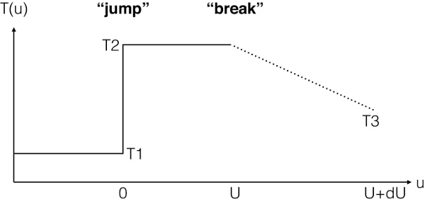
The temperature profile with mode=1.¶

To get the expression for $T(u)$ , we first calculate the increase of the ionisation parameter after $t=t_{\mathrm br}$ as follows:

(2)¶ $\begin{aligned} u-U &=& \int_{t_{\mathrm br}} n(t) dt = \int_{t_{\mathrm br}} n_{\mathrm e} (t/t_{\mathrm br})^{\beta} dt \\ &=& n_{\mathrm e} t_{\mathrm br} ~\int_{1} (t/t_{\mathrm br})^{\beta} ~d(t/t_{\mathrm br}) \\ &=& U / (\beta+1) \cdot [(t/t_{\mathrm br})^{\beta+1} - 1], \end{aligned}$

Then, by combining equations (1) and (2), we obtain:

$\begin{aligned} T(u) = T_2 \cdot [1 + (\beta+1) \cdot (u-U)/U]^{\alpha/(\beta+1)},\end{aligned}$

and we get the final temperature at $u=U+dU$ to be

$\begin{aligned} T_3 = T_2 \cdot [1 + (\beta+1) \cdot dU/U]^{\alpha/(\beta+1)}.\end{aligned}$

It should be noted that, for fixed values of $\alpha$ and $\beta$ , the temperature change after the break is determined by the ratio $dU/U$ rather than $dU$ itself. The user can check $T_3$ with the ascdump plas command (see Ascdump: ascii output of plasma and spectral properties) and also the histories of $u$ and $T(u)$ with the ascdump nei command (see Ascdump: ascii output of plasma and spectral properties).

In some rare cases with a large negative $\beta$ , $T_3$ can get an unphysical value ( $T_3 < 0$ ). In such a case the calculation will automatically be stopped at a lower-limit of $T(u) = 10^{-4}$ keV.

For mode 2, the user may enter an ascii-file with $u$ - and $T$ -values. The format of this file is as follows: the first line contains the number of data pairs ( $u$ , $T$ ). The next lines contain the values of $u$ (in the SPEX units of $10^{20}$ s $\mathrm{m}^{-3}$ ) and $T$ (in keV). Note that $u_1=0$ is a requirement, all $T_i$ should be positive, and the array of $u$ -values should be in ascending order. The pairs ( $u$ , $T$ ) determine the ionisation history, starting from $T=T_1$ (the pre-shock temperature), and the final (radiation) temperature is the temperature of the last bin.

The parameters of the model are:

t1 : Temperature 
before the sudden change in temperature, in keV. Default: 0.002 keV.
t2 : Temperature  after the sudden change in
temperature, in keV. Default: 1 keV.
u : Ionization parameter  before the
“break”, in  m s. Default:
.
du : Ionization parameter  after the “break” in
  s. Default value is 0 (no break).
alfa : Slope  of the  curve after the
“break”. Default value is 0 (constant ).
beta : Slope  of the  curve after the
“break”. Default value is 0 (constant ).
mode : Mode of the model. Mode=1: analytical case; mode=2:
 read from a file. In the latter case, also the parameter
hisu needs to be specified.
hisu : Filename with the  values. Only used when
mode=2.

The following parameters are the same as for the cie-model (Cie: collisional ionisation equilibrium model):

hden : Hydrogen density in  
it : Ion temperature in keV
vrms : RMS Velocity broadening in km/s (see Definition of the micro-turbulent velocity in SPEX)
ref : Reference element
01...30 : Abundances of H to Zn
file : Filename for the nonthermal electron distribution

Recommended citation: Kaastra & Jansen (1993).

4.1.28. Neij: non-equilibrium ionisation jump model¶

Navigation

Related Topics