3.2.8. Plot axis units and scales¶

Different units can be chosen for the quantities that are plotted. Which units are available depends upon the plot type that is used, for example an observed spectrum (data), a Differential Emission Measure distribution (DEM) etc. For the available plot types see Section Plot types.

Note also that depending upon the plot type, there are two or three axes available, the x-axis, y-axis and z-axis. The last axis is only used for contour maps or images, and corresponds to the quantity that is being plotted in the contours or image.

3.2.8.1. X-axis units¶

3.2.8.1.1. X-axis units for plot type model, data, chi, area, fwhm and spec¶

bin	Bin number
kev	keV (kilo-electronvolt), default value
ev	eV (electronvolt)
ryd	Rydberg units
hz	Hertz
ang	Å (Ångstrom)
nm	nm (nanometer)
vel	$\mathrm{km} \ \mathrm{s}^{-1}$

Note: when using the velocity scale, negative values correspond to a blueshift, positive values to a redshift. Also note that in this case one needs to provide the reference energy or wavelength.

3.2.8.1.2. X-axis units for plot type dem¶

bin	Bin number
kev	keV (kilo-electronvolt), default value
ev	eV (electronvolt)
ryd	Rydberg units
k	K (Kelvin)
mk	MK (Mega-Kelvin)

3.2.8.2. Y-axis units¶

3.2.8.2.1. Y-axis units for plot type model, spec¶

	Photon numbers:
cou	$\mathrm{Photons} \ \mathrm{m}^{-2} \mathrm{s}^{-1} \mathrm{bin}^{-1}$
kev	$\mathrm{Photons} \ \mathrm{m}^{-2} \mathrm{s}^{-1} \mathrm{keV}^{-1}$ (default value)
ev	$\mathrm{Photons} \ \mathrm{m}^{-2} \mathrm{s}^{-1} \mathrm{eV}^{-1}$
ryd	$\mathrm{Photons} \ \mathrm{m}^{-2} \mathrm{s}^{-1} \mathrm{Ryd}^{-1}$
hz	$\mathrm{Photons} \ \mathrm{m}^{-2} \mathrm{s}^{-1} \mathrm{Hz}^{-1}$
ang	$\mathrm{Photons} \ \mathrm{m}^{-2} \mathrm{s}^{-1} \mathrm{Å}^{-1}$
nm	$\mathrm{Photons} \ \mathrm{m}^{-2} \mathrm{s}^{-1} \mathrm{nm}^{-1}$
	Energy units:
wkev	$\mathrm{W} \ \mathrm{m}^{-2} \ \mathrm{keV}^{-1}$
wev	$\mathrm{W}\ \mathrm{m}^{-2} \ \mathrm{eV}^{-1}$
wryd	$\mathrm{W}\ \mathrm{m}^{-2} \ \mathrm{Ryd}^{-1}$
whz	$\mathrm{W}\ \mathrm{m}^{-2} \ \mathrm{Hz}^{-1}$
wang	$\mathrm{W}\ \mathrm{m}^{-2} \ \mathrm{Å}^{-1}$
wnm	$\mathrm{W}\ \mathrm{m}^{-2} \ \mathrm{nm}^{-1}$
jans	Jansky ( $10^{-26} \ \mathrm{W}\ \mathrm{m}^{-2} \ \mathrm{Hz}^{-1}$ )
	$\nu F_{\nu}$ units:
iw	$\mathrm{W} \ \mathrm{m}^{-2}$
ij	Jansky Hz ( $10^{-26} \ \mathrm{W}\ \mathrm{m}^{-2}$ )
	Various:
bin	Bin number

3.2.8.2.2. Y-axis units for plot type data¶

bin	Bin number
cou	$\mathrm{Counts}$
cs	$\mathrm{Counts} \ \mathrm{s}^{-1}$
kev	$\mathrm{Counts} \ \mathrm{s}^{-1} \ \mathrm{keV}^{-1}$ (default value)
ev	$\mathrm{Counts} \ \mathrm{s}^{-1} \ \mathrm{eV}^{-1}$
ryd	$\mathrm{Counts} \ \mathrm{s}^{-1} \ \mathrm{Ryd}^{-1}$
hz	$\mathrm{Counts} \ \mathrm{s}^{-1} \ \mathrm{Hz}^{-1}$
ang	$\mathrm{Counts} \ \mathrm{s}^{-1} \ \mathrm{Å}^{-1}$
nm	$\mathrm{Counts} \ \mathrm{s}^{-1} \ \mathrm{nm}^{-1}$
fkev	$\mathrm{Counts} \ \mathrm{m}^{-2} \ \mathrm{s}^{-1} \ \mathrm{keV}^{-1}$
fev	$\mathrm{Counts} \ \mathrm{m}^{-2} \ \mathrm{s}^{-1} \ \mathrm{eV}^{-1}$
fryd	$\mathrm{Counts} \ \mathrm{m}^{-2} \ \mathrm{s}^{-1} \ \mathrm{Ryd}^{-1}$
fhz	$\mathrm{Counts} \ \mathrm{m}^{-2} \ \mathrm{s}^{-1} \ \mathrm{Hz}^{-1}$
fang	$\mathrm{Counts} \ \mathrm{m}^{-2} \ \mathrm{s}^{-1} \ \mathrm{Å}^{-1}$
fnm	$\mathrm{Counts} \ \mathrm{m}^{-2} \ \mathrm{s}^{-1} \ \mathrm{nm}^{-1}$

3.2.8.2.3. Y-axis units for plot type chi¶

bin	Bin number
cou	$\mathrm{Counts}$
cs	$\mathrm{Counts} \ \mathrm{s}^{-1}$
kev	$\mathrm{Counts} \ \mathrm{s}^{-1} \ \mathrm{keV}^{-1}$ (default value)
ev	$\mathrm{Counts} \ \mathrm{s}^{-1} \ \mathrm{eV}^{-1}$
ryd	$\mathrm{Counts} \ \mathrm{s}^{-1} \ \mathrm{Ryd}^{-1}$
hz	$\mathrm{Counts} \ \mathrm{s}^{-1} \ \mathrm{Hz}^{-1}$
ang	$\mathrm{Counts} \ \mathrm{s}^{-1} \ \mathrm{Å}^{-1}$
nm	$\mathrm{Counts} \ \mathrm{s}^{-1} \ \mathrm{nm}^{-1}$
fkev	$\mathrm{Counts} \ \mathrm{m}^{-2} \ \mathrm{s}^{-1} \ \mathrm{keV}^{-1}$
fev	$\mathrm{Counts} \ \mathrm{m}^{-2} \ \mathrm{s}^{-1} \ \mathrm{eV}^{-1}$
fryd	$\mathrm{Counts} \ \mathrm{m}^{-2} \ \mathrm{s}^{-1} \ \mathrm{Ryd}^{-1}$
fhz	$\mathrm{Counts} \ \mathrm{m}^{-2} \ \mathrm{s}^{-1} \ \mathrm{Hz}^{-1}$
fang	$\mathrm{Counts} \ \mathrm{m}^{-2} \ \mathrm{s}^{-1} \ \mathrm{Å}^{-1}$
fnm	$\mathrm{Counts} \ \mathrm{m}^{-2} \ \mathrm{s}^{-1} \ \mathrm{nm}^{-1}$
dchi	(Observed - Model) / Error (default)
rel	(Observed - Model) / Model

3.2.8.2.4. Y-axis units for plot type area¶

bin	Bin number
m2	$\mathrm{m}^2$ (default)
cm2	$\mathrm{cm}^2$

3.2.8.2.5. Y-axis units for plot type fwhm¶

bin	Bin number
kev	keV (kilo-electronvolt), default value
ev	eV (electronvolt)
ryd	Rydberg units
hz	Hertz
ang	Å (Ångstrom)
nm	nm (nanometer)
de/e	$\Delta E / E$

3.2.8.2.6. Y-axis units for plot type dem¶

The emission measure $Y$ is defined as $Y \equiv n_{\mathrm e}n_{\mathrm H}V$ and is expressed in units of $10^{64}$ $\mathrm{m}^{-3}$ . Here $n_{\mathrm e}$ is the electron density, $n_{\mathrm e}$ is the Hydrogen density and $V$ the emitting volume.

bin	Bin number
em	$Y$ (default)
demk	${\mathrm d}Y/{\mathrm d}T$ , per keV
demd	${\mathrm d}Y/{\mathrm d}T$ , per K

3.2.8.3. Plot axis scales¶

The axes in a plot can be plot in different ways, either linear or logarithmic.

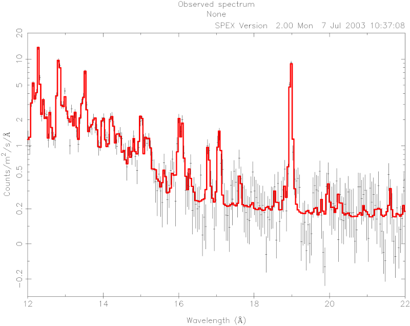
For the y-axis we also have made an option for a mixed linear and logarithmic scale. The lower part of the plot will be on a linear scale, the upper part on a logarithmic scale. This option is useful for example for plotting a background-subtracted spectrum. Often there are bins with a low count rate which scatter around zero after background subtraction; for those channels a linear plot is most suited as a logarithmic scaling cannot deal with negative numbers. On the other hand, other parts of the spectrum may have a high count rate, on various intensity scales, and in that case a logarithmic representation might be optimal. The mixed scaling allows the user to choose below which y-value the plot will be linear, and also which fraction of the plotting surface the linear part will occupy. For an example see the figure below.

Example of the mixed y-axis scale. Simulation of a Chandra LETGS spectrum for a thermal plasma with a temperature of 1 keV.