2.3. Fitting interstellar dust absorption
By: Daniele Rogantini
2.3.1. Goal
Characterise the extinction of the interstellar dust along the line of sight of a bright low-mass X-ray binary observed with Chandra HETG.
Note
This thread merely intends to show the fit of the magnesium and silicon K edges using the amol model. The simulated
dataset with 250 ks exposure time is based on the model used to fit the source GX 3+1 in Rogantini et al. 2019.
2.3.2. Preparation
To follow this thread, it is necessary to download the simulated spectrum and its responsive matrix:
data_sim.spo and data_sim.res.
2.3.3. Starting SPEX
Start SPEX in a linux terminal window:
user@linux:~> spex
Welcome user to SPEX version 3.05.00

SPEX>
2.3.4. Loading data
A command file tailored for this thread to load data is available here data_gx.com:
user@linux:~> cat data_gx.com

# Simulated data
#---------------
# HETG DATA
data data_sim data_sim
bin inst 1 reg 1:2 0:10000 2 unit ang
ignore inst 1 reg 1:2 0:3 unit ang
ignore inst 1 reg 1:2 11:1000 unit ang
Load the above command file into SPEX:
SPEX> log exe data_gx
2.3.5. Plotting data
A command file tailored for this thread to plot the data is available here plot_edges.com:
user@linux:~> cat plot_edges.com
# plot setting
plot dev xw
plot type data
plot x lin
plot y lin
plot ux a
plot uy fa
plot rx 6:10
plot ry 0:900
plot set 1
# HEG color blue
plot data col 11
plot mod lw 3
plot fill disp f
plot back disp f
plot cap id disp f
plot cap ut disp f
plot cap lt disp f
plot
Load the above command file into SPEX:
SPEX> log exe plot_edges
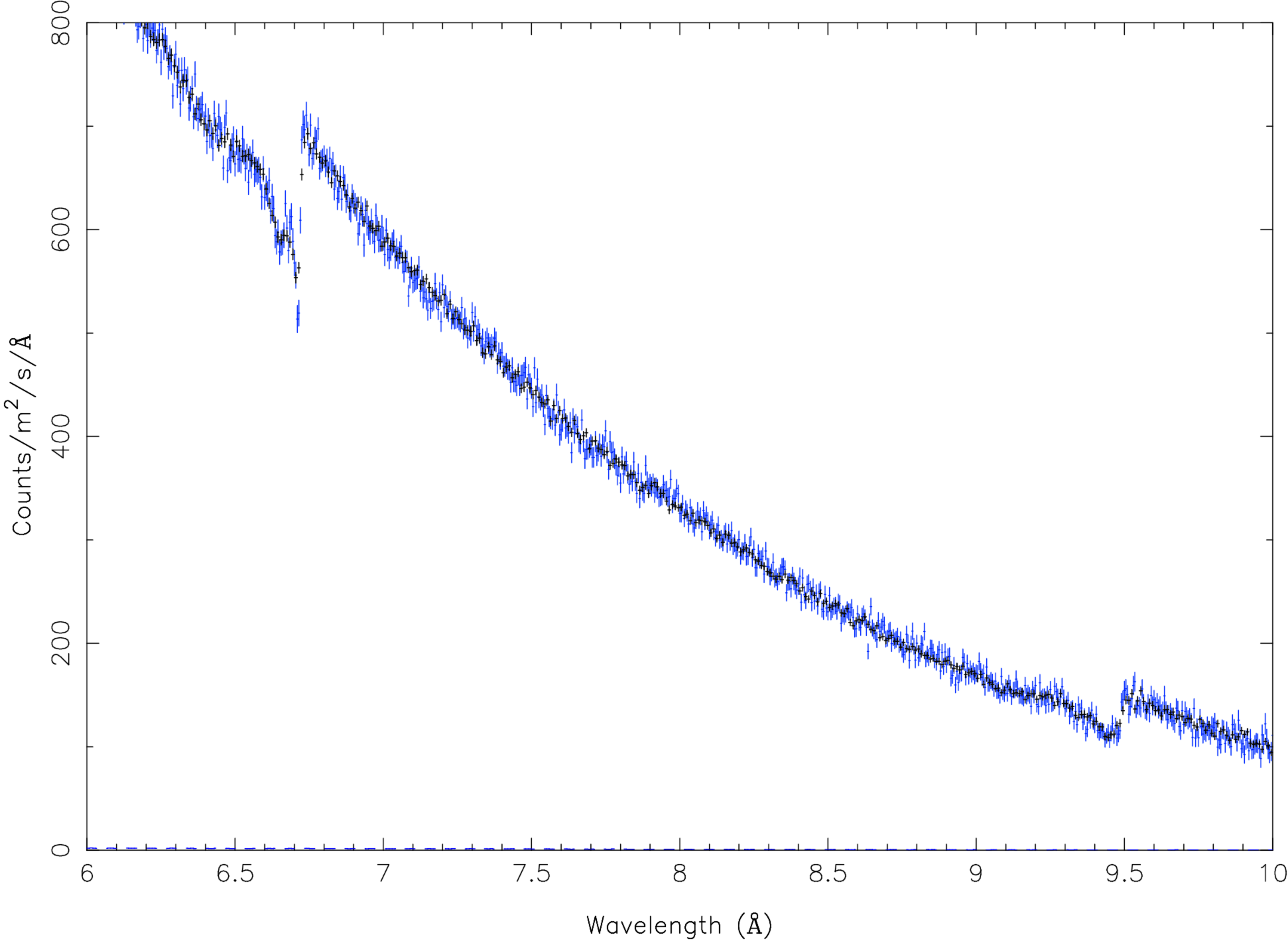
2.3.6. Defining the broadband model
We are studying the interstellar dust along the line of sight of a bright low-mass X-ray binary located near the Galactic bulge (distance 6.1 kpc).
2.3.6.1. Setting the distance of the source
SPEX> distance 6.1 kpc
 Distances assuming H0 =  70.0 km/s/Mpc, Omega_m = 0.300 Omega_Lambda = 0.700 Omega_r = 0.000
Sector       m      A.U.        ly        pc       kpc       Mpc  redshift        cz   age(yr)
----------------------------------------------------------------------------------------------
   1 1.882E+20 1.258E+09 1.990E+04 6100.0000    6.1000 6.100E-03    0.0000       0.4 1.990E+04
----------------------------------------------------------------------------------------------
2.3.6.2. Setting the SED
Set the intrinsic spectral-energy-distribution (SED) of the low-mass X-ray binary. For a typical X-ray binary, the SED between 0.1 and 10 keV is described by two components (Mitsuda et al. 1984): a thermal component, e.g. a black-body (Bb: blackbody model), and a non-thermal component, e.g. a power-law (Pow: power law model):
SPEX> com pow
 You have defined    1 component.
SPEX> par 1 1 norm value 30
SPEX> par 1 1 gamm value 1.1
SPEX> com bb
 You have defined    2 components.
SPEX> par 1 2 norm value 3.e-7
SPEX> par 1 2 t value 0.8
2.3.6.3. Setting the Galactic cold neutral absorption
SPEX> com hot
 You have defined    3 components.
SPEX> par 1 3 nh value 1.9e-2
SPEX> par 1 3 t value 8e-6
SPEX> par 1 3 t status frozen
2.3.7. Defining the dust absorption
Here we introduce the amol components (Amol: interstellar dust absorption model) to characterise the interstellar dust extinction.
In this example we add four arbitrary dust compounds: a-olivine (index=4230,  ),
a-quartz (index=2234,
),
a-quartz (index=2234,  ), c-forsterite (index=3230,
  ), and
a-enstatite (index=3231,
), and
a-enstatite (index=3231,  ). The full list of all compounds is reported in Table
Compounds list and Table Additional compounds list in the Amol: interstellar dust absorption model section of the manual.
). The full list of all compounds is reported in Table
Compounds list and Table Additional compounds list in the Amol: interstellar dust absorption model section of the manual.
2.3.7.1. Setting the interstellar dust models
Defining amol with the initial guess for the column densities of the dust compounds:
SPEX> com amol
 You have defined    4 components.
SPEX> par 1 4 i1 value 4230
SPEX> par 1 4 i2 value 2234
SPEX> par 1 4 i3 value 3230
SPEX> par 1 4 i4 value 3231
SPEX> par 1 4 n1 value 1e-7
SPEX> par 1 4 n2 value 1e-7
SPEX> par 1 4 n3 value 1e-7
SPEX> par 1 4 n4 value 1e-7
SPEX> par 1 4 n1 status thawn
SPEX> par 1 4 n2 status thawn
SPEX> par 1 4 n3 status thawn
SPEX> par 1 4 n4 status thawn
Warning
It is necessary to change and let free to vary the relative abundances of the cold gas elements
(Hot: collisional ionisation equilibrium absorption model in this case) which are also contained in the dust compounds. In this example, the dust models
contain oxygen (08), magnesium (12), silicon (14) and iron (26). We let them to vary within
a limited range according to the depletion intervals defined by
Whittet et al. (2002)
and Jenkins et al. (2009).
SPEX> par 1 3 08 value 0.7
SPEX> par 1 3 12 value 0.10
SPEX> par 1 3 14 value 0.10
SPEX> par 1 3 26 value 0.05
SPEX> par 1 3 08 range 0.4 1
SPEX> par 1 3 12 range 0 0.4
SPEX> par 1 3 14 range 0 0.4
SPEX> par 1 3 26 range 0 0.2
SPEX> par 1 3 08 status thawn
SPEX> par 1 3 12 status thawn
SPEX> par 1 3 14 status thawn
SPEX> par 1 3 26 status thawn
2.3.7.2. Setting the component relations
Adding the multiplicative components hot and amol to the broad-band model:
SPEX> com rel 1:2 4,3
SPEX> model show
--------------------------------------------------------------------------------
 Number of sectors         :     1
 Sector:    1 Number of model components:     4
    Nr.    1: pow [4,3 ]
    Nr.    2: bb  [4,3 ]
    Nr.    3: hot
    Nr.    4: amol
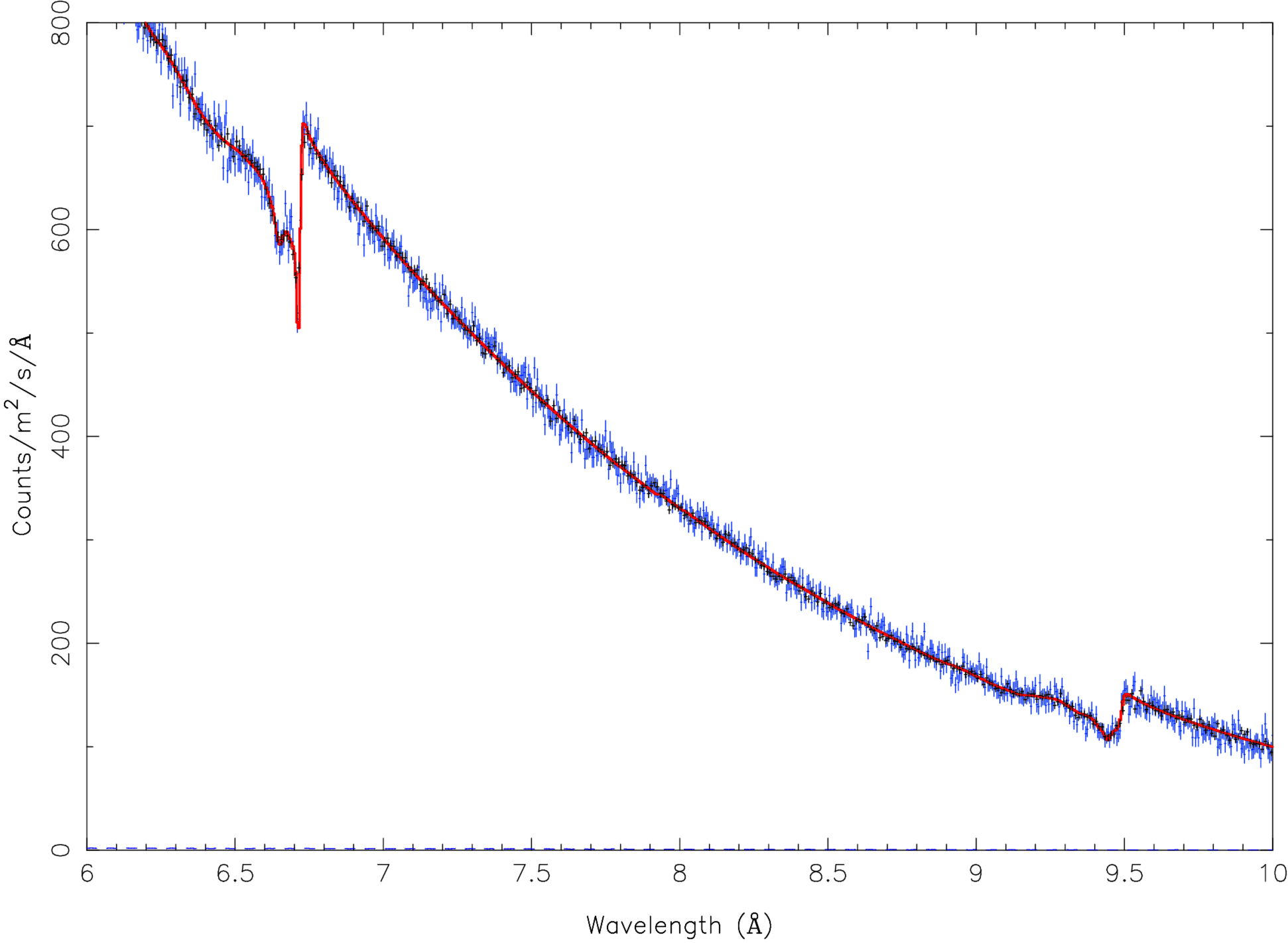
2.3.8. Fitting
We fit the model to the data and print the free parameters:
SPEX> calc
SPEX> fit print 1
SPEX> fit
SPEX> fit
SPEX> plot
SPEX> par show free

--------------------------------------------------------------------------------------------------
sect comp mod  acro parameter with unit     value      status    minimum   maximum lsec lcom lpar

   1    1 pow  norm Norm (1E44 ph/s/keV)  23.14066     thawn     0.0      1.00E+20
   1    1 pow  gamm Photon index         0.9320605     thawn    -10.       10.

   1    2 bb   norm Area (1E16 m**2)     3.5883755E-07 thawn     0.0      1.00E+20
   1    2 bb   t    Temperature (keV)    0.7793768     thawn    1.00E-04  1.00E+03

   1    3 hot  nh   X-Column (1E28/m**2) 2.0304110E-02 thawn     0.0      1.00E+20
   1    3 hot  08   Abundance O          0.5010648     thawn    0.40       1.0
   1    3 hot  12   Abundance Mg         0.1016048     thawn     0.0      0.40
   1    3 hot  14   Abundance Si         0.1060375     thawn     0.0      0.40
   1    3 hot  26   Abundance Fe          0.000000     thawn     0.0      0.20

   1    4 amol n1   Column 1 (1E28/m**2) 5.6286910E-07 thawn     0.0      1.00E+20
   1    4 amol n2   Column 1 (1E28/m**2) 1.1466740E-07 thawn     0.0      1.00E+20
   1    4 amol n3   Column 1 (1E28/m**2) 1.3037014E-07 thawn     0.0      1.00E+20
   1    4 amol n4   Column 1 (1E28/m**2) 9.8849377E-08 thawn     0.0      1.00E+20


Instrument     1 region    1 has norm    1.00000E+00 and is frozen
Instrument     1 region    2 has norm    1.00000E+00 and is frozen

--------------------------------------------------------------------------------
 Fluxes and restframe luminosities between   2.0000     and    10.000     keV

 sect comp mod   photon flux   energy flux nr of photons    luminosity
              (phot/m**2/s)      (W/m**2)   (photons/s)           (W)
    1    1 pow    7877.93      6.754451E-12  4.125361E+45  3.331746E+30
    1    2 bb     3030.35      1.681985E-12  1.818740E+45  9.538203E+29

--------------------------------------------------------------------------------
 Fit method        : Classical Levenberg-Marquardt
 Fit statistic     : C-statistic
 C-statistic       :      2388.02
 Expected C-stat   :      2402.60 +/-        69.35
 Chi-squared value :      2406.15
 Degrees of freedom:      2388
 W-statistic       :         0.00
2.3.9. Final remarks
This is the end of this analysis thread. If you want, you can save the parameters and quit SPEX:
SPEX> par write parameters
SPEX> log out fit_result
SPEX> par show
SPEX> log close output
    SPEX> quit
     Thank you for using SPEX!