2.2. Modeling particle background

2.2.1. Goal

Time dependent particle backgrounds in X-ray spectra are very difficult to correctly subtract, especially for extended sources. Many times, a quiescent particle background remains present in the spectrum after flare filtering. In this example, we show how to model the quiescent soft-proton contribution in a spectrum extracted from an annulus around the core of a cluster of galaxies. The difficulty here is that the effective area for soft protons is very different from the effective area for X-rays. Please note that the example provided is not necessarily scientifically correct. The goal of this example is to show a general method to deal with these kind of problems in SPEX. The choice of models probably needs to be different in other cases.

2.2.2. SPEX solution

The basic problem we have to solve here, is that we need a number of model components that are folded through the mirror effective area (the cosmic X-rays) and a few components describing the particle background, which are not folded through the ARF. In SPEX, this can be solved using sectors (Sectors and regions). Sectors are essentially model groups representing different areas or different components on the sky. In this case, we will create two sectors: one for the cosmic X-rays and one for the particle background. The second sector should not be folded through the ARF. To achieve this, we have to create a special spectrum and response file with trafo (Trafo) in which we define the sectors.

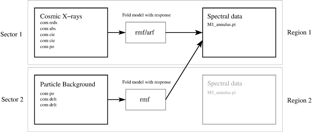
Schematic representation of the sectors and regions in this example. We load two spectra with trafo and we define two sectors (left). The exact model components are later defined in SPEX. The models for sectors 1 and 2 are folded through the response matrix separately. The result of the folding is added and applied to the first spectrum (region 1 on the right) only.

2.2.2.1. Running trafo

In this trafo run, we will actually load the same spectrum twice. One for every sector. Here we use a MOS1 spectrum extracted from an annulus between 6 and 9 arcmin from the cluster core. The background spectrum was extracted using the XMM Extended Source Analysis Software by Snowden & Kuntz. After starting trafo we have to tell it that we want to transform two spectra in two sectors:

Program trafo: transform data to SPEX 2.0 format
This is version 1.02, of trafo

 Are your data in OGIP format            : type=1
 Old (Version 1.10 and below) SPEX format: type=2

 Enter the type: 1
 Enter the number of spectra you want to transform: 2
 Enter the maximum number of response groups per energy per spectrum: 1000000
 Enter the number of sectors you want to create: 2

The region number respresents the spectral data that we will fit. Because we want to add the cosmic X-ray spectrum and the particle background spectrum, we want both sectors to point to region 1. First, we enter the spectra for the first sector. We only show the most relevant input/output lines here.

Enter the sector and region number: 1 1
How should the matrix be partioned?
Option 1: keep as provided (1 component, no re-arrangements)
Option 2: rearrange into contiguous groups
Option 3: split into N roughly equal-sized components
Enter your preferred option (1,2,3): 1
Enter filename spectrum to be read: M1_annulus.pi
Read nevertheless a background file? (y/n) [no]: y
Enter filename background spectrum to be read: M1_annulus_bkg.pi
Shall we ignore bad channels? (y/n) [no]:y
Enter filename response matrix to be read: M1_annulus.rmf
Enter new bin boundary values manually: 3.E-5 5.E-3
Enter shift to response array (1 recommended, but some cases may be 0):1
Read nevertheless an effective area file? (y/n) [no]: y
Enter filename arf-file to be read: M1_annulus.arf

The first spectrum is now read in, including an ARF file. Now we enter the same spectrum again, but now without ARF. The region number here is 1, because we want the models in this sector to be added to the models of sector 1.

Enter the sector and region number: 2 1
Enter your preferred option (1,2,3): 1
Enter filename spectrum to be read: M1_annulus.pi
Read nevertheless a background file? (y/n) [no]: y
Enter filename background spectrum to be read: M1_annulus_bkg.pi
Enter filename response matrix to be read: M1_annulus.rmf
Read nevertheless an effective area file? (y/n) [no]: n

Save the spectrum by providing convenient names for the res and spo files.

Enter filename spectrum to be saved (without .spo): M1_annulus
Enter filename response to be saved (without .res): M1_annulus

2.2.2.2. Running SPEX

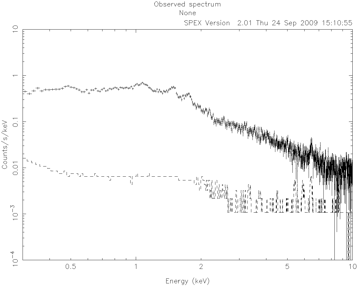
XMM-Newton MOS1 spectrum extracted from a 6–9 arcmin annulus around a cluster of galaxies.

If the res and spo files are created, we are ready to run spex. In this description, we skip some very basic commands about, for example, plotting. See How to run SPEX for an overview of a basic SPEX session. First, we load the spectrum and plot it:

 Welcome user to SPEX version 3.00.00

SPEX> data M1_annulus M1_annulus
...
SPEX> plot

Figure XMM-Newton MOS1 spectrum extracted from a 6–9 arcmin annulus around a cluster of galaxies. shows a plot of the spectrum. For presentation purposes we rebin the spectrum here with the obin command (Obin: optimal rebinning of the data). If C-statistics are used, binning is not strictly necessary. An important thing to remember at this point is to ignore the spectrum in region number 2:

SPEX> ign reg 2 1:1000000

We ignore region 2 from channel 1 to 1000000, which should be more then enough to make sure no data is left in the region. Of course, some data at very low and high energies also need to be ignored in region 1.

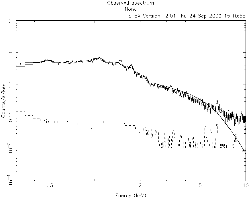
A fit without modeling the particle background is not successful. Especially, the high-energy region in the spectrum is not fitted well due to soft protons.

Now, we set up the cosmic X-ray model for sector 1. We can just load the components normally, because they are automatically added to the first sector:

SPEX> com reds
SPEX> com abs
SPEX> com cie
SPEX> com cie
SPEX> com po
SPEX> com rel 3 1,2
SPEX> com rel 5 1,2

In this model, we put a cosmological redshift, interstellar absorption, and a single-temperature model to describe the cluster emission. In addition, we put a single-temperature model with a fixed temperature of 0.2 keV to model the emission from the local hot bubble, and a power law with a gamma value of 1.41 to account for the Cosmic X-ray Backgound (CXB) due to unresolved point sources.

SPEX> par 1 4 t v 0.2
SPEX> par 1 4 t s f
SPEX> par 1 5 gamm v 1.41
SPEX> par 1 5 gamm s f

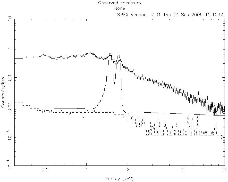
Here, we plot the particle background model. We ignore the cluster model components for now. It is clear to see that the power law is not folded through the arf.

Just to show what happens if we fit the data now, we plot the result in Figure A fit without modeling the particle background is not successful. Especially, the high-energy region in the spectrum is not fitted well due to soft protons.. It is clear that the spectrum is not well fitted at low and high energies. A contribution of soft protons is visible at the high-energy end of the spectrum. In addition, we see that the instrumental fluoresence lines of Al and Si at 1.49 and 1.75 keV are not fitted. To model these features, we need to use the second sector and define an additional model there.

SPEX> sector new
SPEX> com 2 po
SPEX> com 2 delt
SPEX> com 2 delt
SPEX> par 2 1 gamm v 0.2
SPEX> par 2 2 e v 1.49
SPEX> par 2 2 e s f
SPEX> par 2 3 e v 1.75
SPEX> par 2 3 e s f

In this sequence of commands, we define a new sector (number 2) and add a power-law and two delta-line components to it. The slope of the gamma-parameter is initially set to 0.2. In Figure Here, we plot the particle background model. We ignore the cluster model components for now. It is clear to see that the power law is not folded through the arf., we put the components in sector 1 to zero to show the particle background model that we have just defined. The flat shape of the power-law model confirms that these components are not folded through the arf.

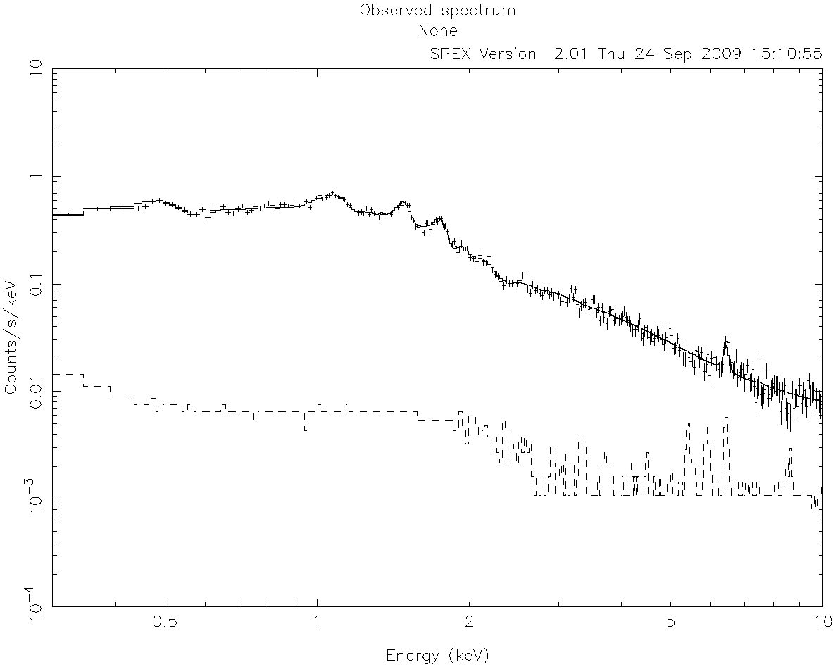
Best fit model to our example spectrum. The particle background model has been able to fit the discrepancies at high energies.

When we reset the components in sector 1 to their initial values we can start fitting. In Figure Best fit model to our example spectrum. The particle background model has been able to fit the discrepancies at high energies., we show the best fit using this model. The contribution of soft-protons at high energies is now being accounted for by the power law.

Warning

The example above uses a simplified model of the X-ray background. Background subtraction for extended sources is complicated and subject of continuous research. Please be very careful in selecting model components and deciding which parameters can be left free.