2.1. Fitting a CCD spectrum
2.1.1. Goal
To load and fit a CCD spectrum (e.g. MOS1 aboard XMM-Newton) into SPEX.
2.1.2. Preparation
To be able to fit a spectrum, you need a spectrum and response file in SPEX format. To convert spectra from OGIP
format (e.g. pha, arf, rmf) to SPEX format, please use the trafo program like described in How to convert spectra to SPEX format.
If you have the Pyspextools package installed, then you can use
ogip2spex as an alternative to trafo.
Using the commands above, you can obtain a .spo and .res file containing your spectrum. To follow this thread, you
can also download example files here: mos.spo and mos.res.
2.1.3. Starting SPEX
The SPEX program is started by entering spex in a linux terminal window. In the following sections we describe
one run of the program. To start SPEX do this:
user@linux:~> spex
 Welcome user to SPEX version 3.06.00

SPEX>
If SPEX does not run, please check if you set the SPEX90 variable right and sourced spexdist.(c)sh
as explained in How to install SPEX.
2.1.4. Loading data
Then, we have to load the data files. This is done using the data command (Data: read response file and spectrum). It is a general thing
in SPEX that filename extensions are not typed explicitly when issuing a command. If you have a file called
mos.spo and mos.res then you type:
SPEX> data mos mos
The response file (mos.res) is entered first and then the file containing the spectrum (mos.spo). You can avoid
confusion by giving the same filename to both .res and .spo files. Remember that the order of the words in the commands
is very important!
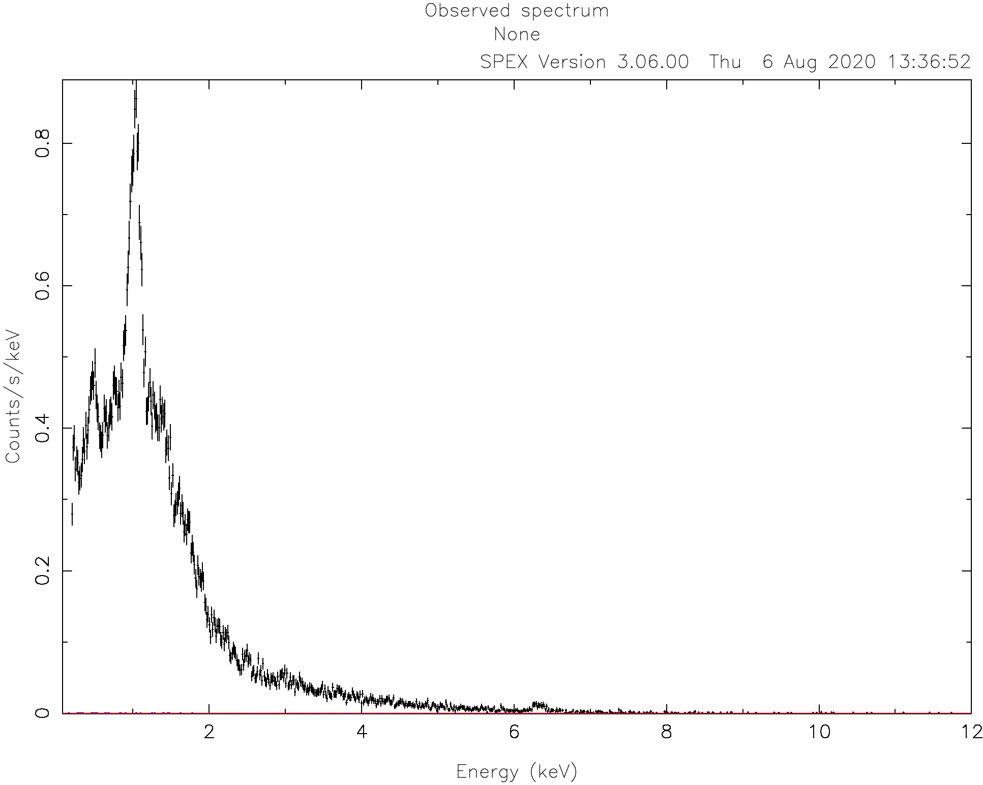
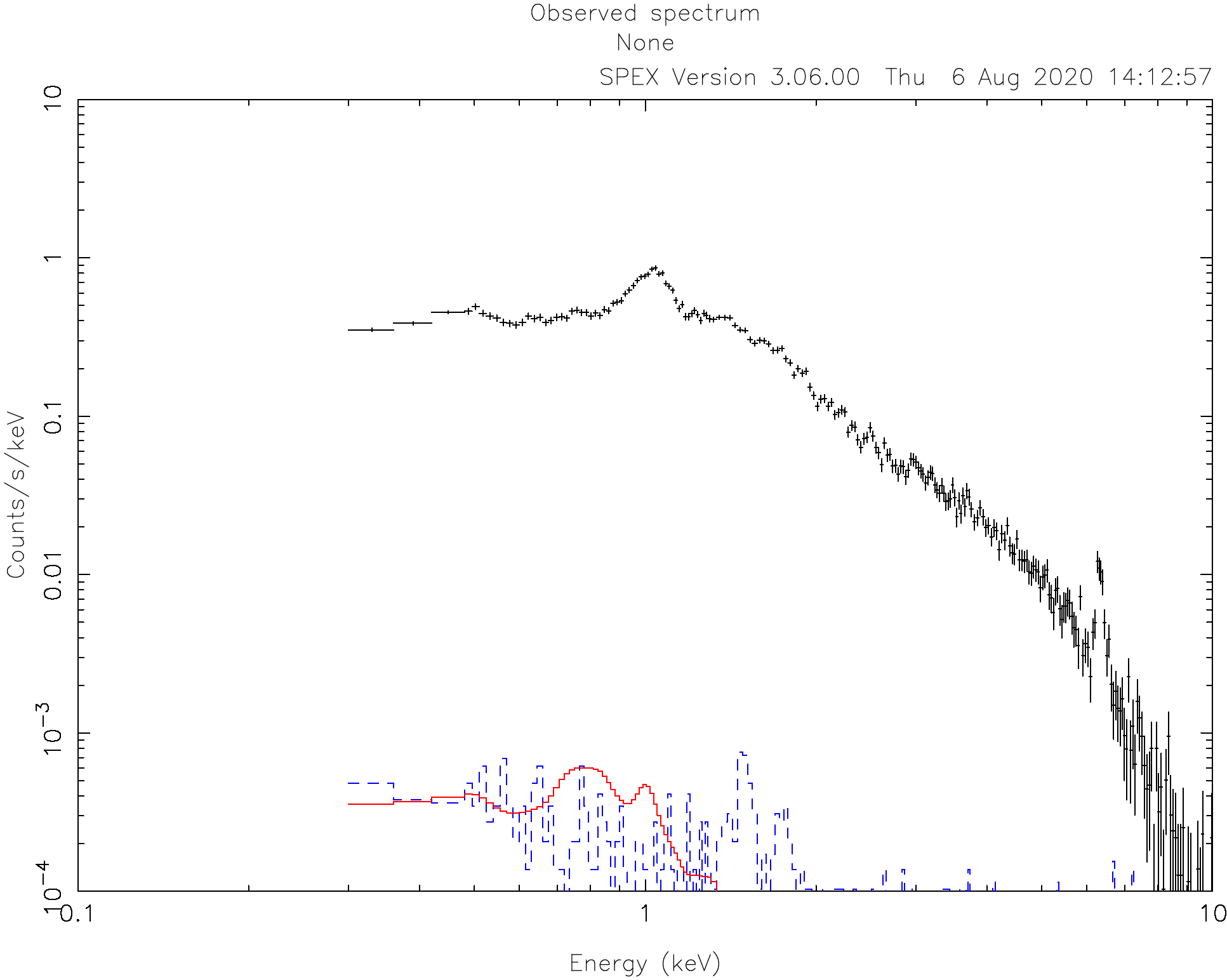
2.1.5. Plot the data
It really helps to see the spectrum while we are working on it, so we need a plot window and tell spex that we want to see a plot of the data. (Note that the text after the # is a comment and should not be copied on the command line).
SPEX> plot dev xs             # Open plot device `X server`
SPEX> plot type data          # Choose the plot type `data`
SPEX> plot
The commands above open a PGPLOT window and set the plot type to data, which means that the observed spectrum
and the model (folded through the response matrix) will be shown. The last plot command tells SPEX to
refresh the plot.
Usually CCD spectra benefit from a logarithmic scale on both the X and Y axes:
SPEX> plot x log
SPEX> plot y log
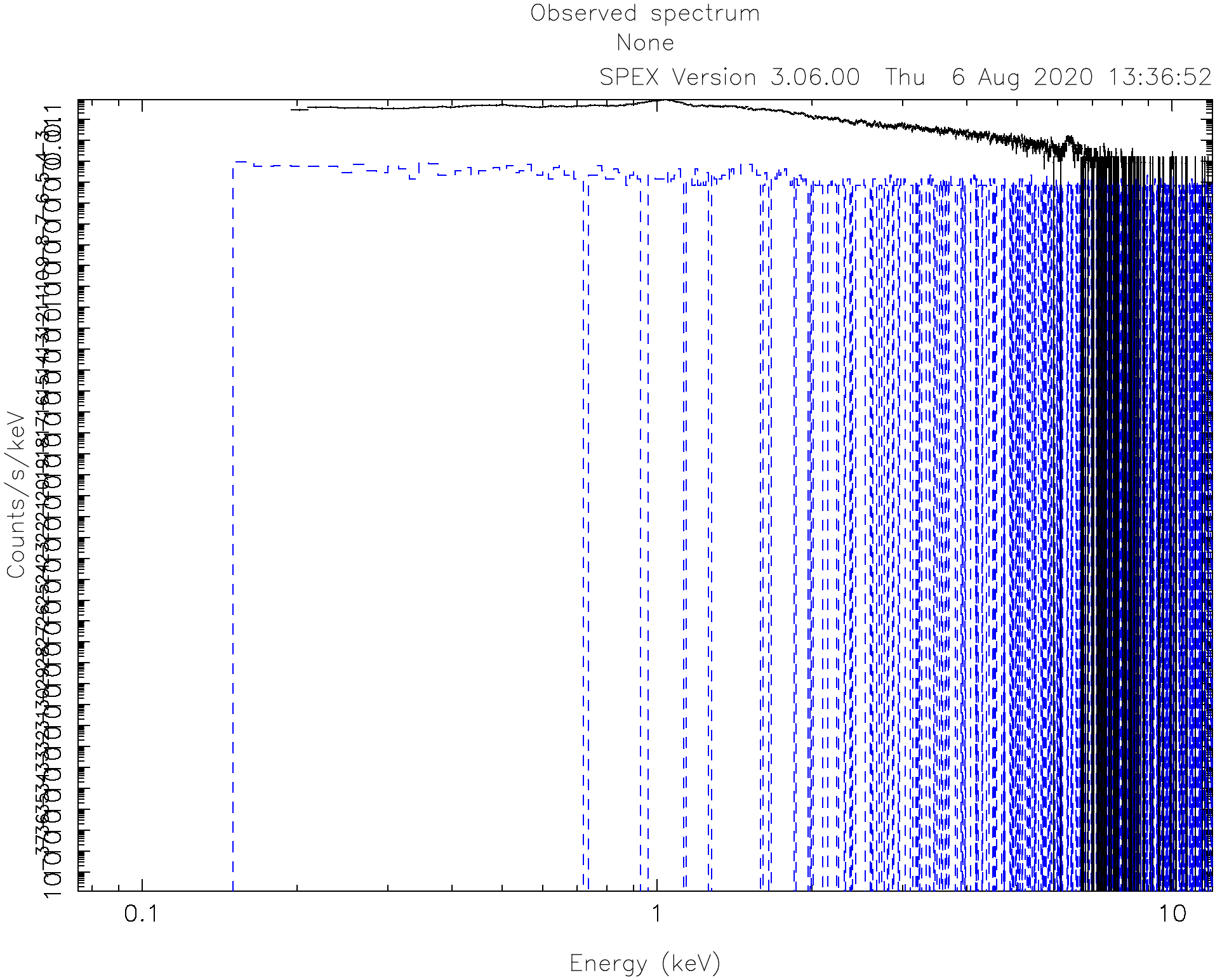
By default, the ranges of the axes are usually too broad. For this spectrum, the X axis range is good between 0.1 and 10 keV and the Y axis range between 1E-4 and 10.
SPEX> plot rx 0.1:10.
SPEX> plot ry 1E-4:10.
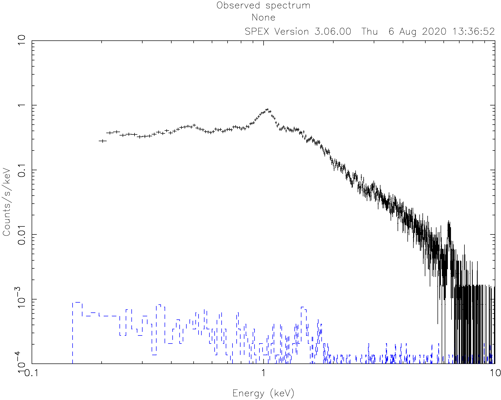
2.1.6. Select good data and bin the spectrum
Before we start fitting, we can make sure that only trustworthy data is fitted. For MOS1, for example, we know that
the calibration is valid for the energy range between roughly 0.3 keV and 10 keV. To fit only the good spectral
interval, we need to ignore the parts at low and high energies. This is done using the ignore command.
In addition, we can bin the spectrum. To automatically rebin to the recommended (optimal) bin size, one can use
the obin command. This command bins the spectrum optimally based on the instrument resolution and statistics.
SPEX> ignore 0:0.3 unit kev
SPEX> ignore 10:100 unit kev
SPEX> obin 0.3:10 unit kev
SPEX> plot
2.1.7. Define the model
Next we can define the model that we want to fit. In this case, we are looking at a MOS spectrum of a
galaxy cluster. The simplest model that we can try is a single temperature spectrum absorbed by gas in
the ISM. We also add a redshift component reds (Reds: redshift model) to shift the energy of the model
spectrum with the right amount:
SPEX> com reds
You have defined    1 component.
SPEX> com hot
You have defined    2 components.
SPEX> com cie
You have defined    3 components.
The hot model (Hot: collisional ionisation equilibrium absorption model) is actually a gas in equilibrium in absorption, which is a fair representation of
the neutral gas phase of the ISM. Later we will put the temperature of this component to  keV
to emulate a neutral plasma.
keV
to emulate a neutral plasma.
The cie model (Cie: collisional ionisation equilibrium model) represents a single temperature plasma in collisional ionisation equilibrium,
which is commonly used for clusters.
Then the components need to be related to each other, which means you need to specify how the multiplicative models should be applied to the additive models. The multiplicative components should be listed in order from the source to the observer (see also Comp: create, delete and relate spectral components):
SPEX> com rel 3 1,2
This means that the emitted CIE component (#3) will be first redshifted by component #1 and then absorbed by component #2. If you have multiple additive components, this should be done for each one. It is possible to supply a range of components.
SPEX> calc
SPEX> plot
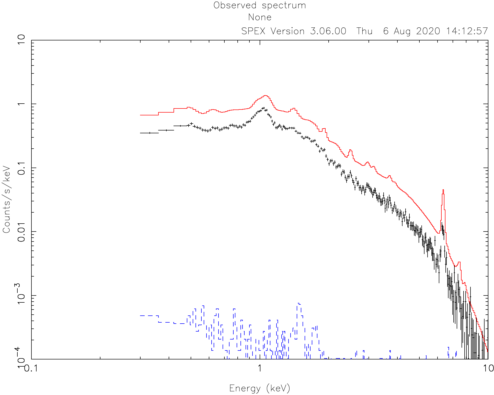
Calculating and plotting the model unsurprisingly results in a curve that is not near to the data.
2.1.8. Initial guess of parameters
To help the spectral fitting process, it is good to provide initial guesses for the model parameters. This way, the spectral fit starts already with a model that is in the right direction. As a more experienced user, you usually have a rough idea what the parameters should be by looking at the raw spectrum. For this cluster, for example, the redshift is around 0.05, the absorption column is small, and the temperature of the cluster is around 3 keV. We can set the guess parameters as follows:
SPEX> par 1 1 z v 0.05
SPEX> par 1 1 z s t
SPEX> par 1 2 t v 8E-6
SPEX> par 1 2 t s f
SPEX> par 1 2 nh v 1E-4
SPEX> par 1 3 norm v 1000.
SPEX> par 1 3 t v 3.0
SPEX> ca
SPEX> pl
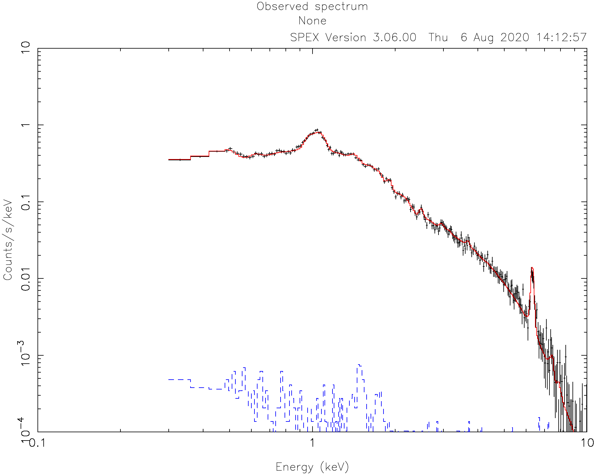
As we can see from the image, the first guess of the model is already in the right direction.
In this example, we assume that the exact redshift is unknown. However, if you do have an accurate measurement of the distance, it is wise to set that distance in SPEX (Distance: set the source distance):
SPEX> dist 0.05 z
The command above sets the distance to 0.05 z and makes sure that the luminosities are correctly calculated. Note that this distance change also affects the values of the normalisation of the models! So, we increase the normalisation to keep the model reasonably close to the data:
SPEX> par 1 3 norm v 1E+8
2.1.9. Fit the model
We are now ready to fit the spectrum. To see the fitting steps, we can give the command fit print 1. This needs
to be set only once per session. A subsequent fit command (Fit: spectral fitting) starts to optimize the parameters:
SPEX> fit print 1
SPEX> fit
   42102.6              5  5.000E-02  1.000E-04  1.000E+08   3.00
   2461.87             10  5.404E-02  9.087E-05  2.021E+08   2.04
   428.533             15  5.439E-02  1.041E-04  2.412E+08   2.31
   414.925             20  5.437E-02  9.425E-05  2.429E+08   2.37
   414.651             25  5.426E-02  9.229E-05  2.428E+08   2.37
   414.532             30  5.408E-02  9.269E-05  2.428E+08   2.37
   414.525             35  5.412E-02  9.281E-05  2.428E+08   2.37
   414.524             42  5.411E-02  9.270E-05  2.428E+08   2.37
   414.524             48  5.411E-02  9.265E-05  2.428E+08   2.37
--------------------------------------------------------------------------------------------------
sect comp mod  acro parameter with unit     value      status    minimum   maximum lsec lcom lpar

   1    1 reds z    Redshift             5.4108180E-02 thawn    -1.0      1.00E+10
   1    1 reds flag Flag: cosmo=0, vel=1  0.000000     frozen    0.0       1.0

   1    2 hot  nh   X-Column (1E28/m**2) 9.2653019E-05 thawn     0.0      1.00E+20
   1    2 hot  t    Temperature (keV)    1.9999999E-04 frozen   2.00E-04  1.00E+03
   1    2 hot  rt   T(balance) / T(spec)  1.000000     frozen   1.00E-04  1.00E+04
   1    2 hot  fcov Covering fraction     1.000000     frozen    0.0       1.0
   1    2 hot  v    RMS Velocity (km/s)   100.0000     frozen    0.0      3.00E+05
   1    2 hot  rms  RMS blend    (km/s)   0.000000     frozen    0.0      1.00E+05
   1    2 hot  dv   Vel. separ. (km/s)    100.0000     frozen    0.0      1.00E+05
   1    2 hot  zv   Average vel. (km/s)   0.000000     frozen  -1.00E+05  1.00E+05
   1    2 hot  ref  Reference atom        1.000000     frozen    1.0       30.
   1    2 hot  01   Abundance H           1.000000     frozen    0.0      1.00E+10
   1    2 hot  02   Abundance He          1.000000     frozen    0.0      1.00E+10
   1    2 hot  03   Abundance Li          1.000000     frozen    0.0      1.00E+10
   1    2 hot  04   Abundance Be          1.000000     frozen    0.0      1.00E+10
   1    2 hot  05   Abundance B           1.000000     frozen    0.0      1.00E+10
   1    2 hot  06   Abundance C           1.000000     frozen    0.0      1.00E+10
   1    2 hot  07   Abundance N           1.000000     frozen    0.0      1.00E+10
   1    2 hot  08   Abundance O           1.000000     frozen    0.0      1.00E+10
   1    2 hot  09   Abundance F           1.000000     frozen    0.0      1.00E+10
   1    2 hot  10   Abundance Ne          1.000000     frozen    0.0      1.00E+10
   1    2 hot  11   Abundance Na          1.000000     frozen    0.0      1.00E+10
   1    2 hot  12   Abundance Mg          1.000000     frozen    0.0      1.00E+10
   1    2 hot  13   Abundance Al          1.000000     frozen    0.0      1.00E+10
   1    2 hot  14   Abundance Si          1.000000     frozen    0.0      1.00E+10
   1    2 hot  15   Abundance P           1.000000     frozen    0.0      1.00E+10
   1    2 hot  16   Abundance S           1.000000     frozen    0.0      1.00E+10
   1    2 hot  17   Abundance Cl          1.000000     frozen    0.0      1.00E+10
   1    2 hot  18   Abundance Ar          1.000000     frozen    0.0      1.00E+10
   1    2 hot  19   Abundance K           1.000000     frozen    0.0      1.00E+10
   1    2 hot  20   Abundance Ca          1.000000     frozen    0.0      1.00E+10
   1    2 hot  21   Abundance Sc          1.000000     frozen    0.0      1.00E+10
   1    2 hot  22   Abundance Ti          1.000000     frozen    0.0      1.00E+10
   1    2 hot  23   Abundance V           1.000000     frozen    0.0      1.00E+10
   1    2 hot  24   Abundance Cr          1.000000     frozen    0.0      1.00E+10
   1    2 hot  25   Abundance Mn          1.000000     frozen    0.0      1.00E+10
   1    2 hot  26   Abundance Fe          1.000000     frozen    0.0      1.00E+10
   1    2 hot  27   Abundance Co          1.000000     frozen    0.0      1.00E+10
   1    2 hot  28   Abundance Ni          1.000000     frozen    0.0      1.00E+10
   1    2 hot  29   Abundance Cu          1.000000     frozen    0.0      1.00E+10
   1    2 hot  30   Abundance Zn          1.000000     frozen    0.0      1.00E+10
   1    2 hot  file File electr.distrib.

   1    3 cie  norm ne nX V (1E64/m**3)  2.4279381E+08 thawn     0.0      1.00E+20
   1    3 cie  t    Temperature (keV)     2.372914     thawn    5.00E-04  1.00E+03
   1    3 cie  sig  Sigma                 0.000000     frozen    0.0      1.00E+04
   1    3 cie  sup  Sigma up              0.000000     frozen    0.0      1.00E+04
   1    3 cie  logt T grid (lin/log)      1.000000     frozen    0.0       1.0
   1    3 cie  ed   El  dens (1E20/m**3) 9.9999998E-15 frozen   1.00E-22  1.00E+10
   1    3 cie  it   Ion temp  (keV)       1.000000     frozen   1.00E-04  1.00E+07
   1    3 cie  rt   T(balance) / T(spec)  1.000000     frozen   1.00E-04  1.00E+04
   1    3 cie  vrms RMS Velocity (km/s)   0.000000     frozen    0.0      3.00E+05
   1    3 cie  ref  Reference atom        1.000000     frozen    1.0       30.
   1    3 cie  01   Abundance H           1.000000     frozen    0.0      1.00E+10
   1    3 cie  02   Abundance He          1.000000     frozen    0.0      1.00E+10
   1    3 cie  03   Abundance Li          1.000000     frozen    0.0      1.00E+10
   1    3 cie  04   Abundance Be          1.000000     frozen    0.0      1.00E+10
   1    3 cie  05   Abundance B           1.000000     frozen    0.0      1.00E+10
   1    3 cie  06   Abundance C           1.000000     frozen    0.0      1.00E+10
   1    3 cie  07   Abundance N           1.000000     frozen    0.0      1.00E+10
   1    3 cie  08   Abundance O           1.000000     frozen    0.0      1.00E+10
   1    3 cie  09   Abundance F           1.000000     frozen    0.0      1.00E+10
   1    3 cie  10   Abundance Ne          1.000000     frozen    0.0      1.00E+10
   1    3 cie  11   Abundance Na          1.000000     frozen    0.0      1.00E+10
   1    3 cie  12   Abundance Mg          1.000000     frozen    0.0      1.00E+10
   1    3 cie  13   Abundance Al          1.000000     frozen    0.0      1.00E+10
   1    3 cie  14   Abundance Si          1.000000     frozen    0.0      1.00E+10
   1    3 cie  15   Abundance P           1.000000     frozen    0.0      1.00E+10
   1    3 cie  16   Abundance S           1.000000     frozen    0.0      1.00E+10
   1    3 cie  17   Abundance Cl          1.000000     frozen    0.0      1.00E+10
   1    3 cie  18   Abundance Ar          1.000000     frozen    0.0      1.00E+10
   1    3 cie  19   Abundance K           1.000000     frozen    0.0      1.00E+10
   1    3 cie  20   Abundance Ca          1.000000     frozen    0.0      1.00E+10
   1    3 cie  21   Abundance Sc          1.000000     frozen    0.0      1.00E+10
   1    3 cie  22   Abundance Ti          1.000000     frozen    0.0      1.00E+10
   1    3 cie  23   Abundance V           1.000000     frozen    0.0      1.00E+10
   1    3 cie  24   Abundance Cr          1.000000     frozen    0.0      1.00E+10
   1    3 cie  25   Abundance Mn          1.000000     frozen    0.0      1.00E+10
   1    3 cie  26   Abundance Fe          1.000000     frozen    0.0      1.00E+10
   1    3 cie  27   Abundance Co          1.000000     frozen    0.0      1.00E+10
   1    3 cie  28   Abundance Ni          1.000000     frozen    0.0      1.00E+10
   1    3 cie  29   Abundance Cu          1.000000     frozen    0.0      1.00E+10
   1    3 cie  30   Abundance Zn          1.000000     frozen    0.0      1.00E+10
   1    3 cie  file File electr.distrib.
   1    3 cie  x1   T1/T0                 1.000000     frozen    1.0      1.00E+10
   1    3 cie  y1   N1/N0                 0.000000     frozen    0.0      1.00E+10


Instrument     1 region    1 has norm    1.00000E+00 and is frozen

--------------------------------------------------------------------------------
 Fluxes and restframe luminosities between   2.0000     and    10.000     keV

 sect comp mod   photon flux   energy flux nr of photons    luminosity
              (phot/m**2/s)      (W/m**2)   (photons/s)           (W)
    1    3 cie    4.13667      2.229383E-15  2.655905E+51  1.422295E+36

--------------------------------------------------------------------------------
 Fit method        : Classical Levenberg-Marquardt
 Fit statistic     : C-statistic
 C-statistic       :       414.52
 Expected C-stat   :       247.13 +/-        21.92
 Chi-squared value :       528.16
 Degrees of freedom:       239
 W-statistic       :         0.00
At the end of the optimization step, SPEX prints out an overview of the fit parameters and the fit statistics. Here we can see that the fit improved, but there is still room for improvement.

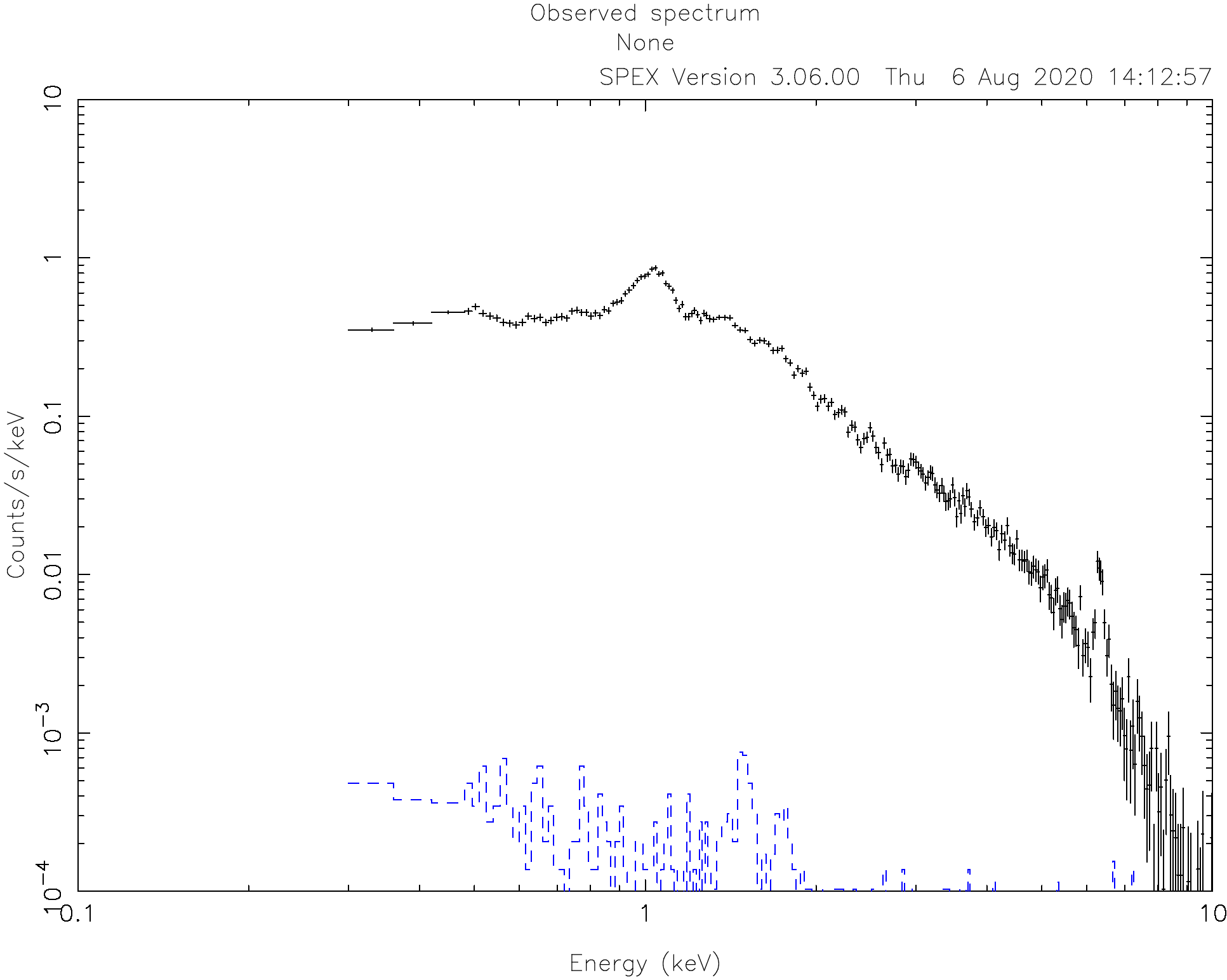
2.1.10. Fitting abundances
Although the C-statistics are not too bad, there are still residuals in the spectrum, especially around the strongest spectral lines. This is because the metal abundances in the gas are still fixed to 1.0. We can let the abundances vary in the optimization by setting them to thawn:
SPEX> par 1 3 08 s t
SPEX> par 1 3 12 s t
SPEX> par 1 3 14 s t
SPEX> par 1 3 16 s t
SPEX> par 1 3 18 s t
SPEX> par 1 3 20 s t
SPEX> par 1 3 26 s t
SPEX> par 1 3 28 s t
SPEX> fit
The optimization leads to an even better fit:
Fit method        : Classical Levenberg-Marquardt
Fit statistic     : C-statistic
C-statistic       :       266.80
Expected C-stat   :       247.12 +/-        21.91
Chi-squared value :       366.77
Degrees of freedom:       231
W-statistic       :         0.00
2.1.11. Calculating errors
When we have the best fit, we can calculate the errors (Error: Calculate the errors of the fitted parameters). This has to be done per parameter. Below we calculate, for example, the error on the best fit temperature:
SPEX> error 1 3 t
 parameter          C-stat      Delta          Delta
   value            value       parameter     C-stat
----------------------------------------------------
   2.33348          267.68     -2.246547E-02    0.89
   2.31101          270.23     -4.493093E-02    3.44
   2.33348          267.68     -2.246547E-02    0.89
   2.33247          267.69     -2.346587E-02    0.90
   2.32425          268.52     -3.169394E-02    1.73
   2.32836          268.05     -2.758002E-02    1.26
   2.33042          267.87     -2.552295E-02    1.07
   2.33127          267.79     -2.466774E-02    1.00
   2.37841          267.71      2.246547E-02    0.92
   2.40087          270.28      4.493093E-02    3.49
   2.37841          267.71      2.246547E-02    0.92
   2.37914          267.77      2.319646E-02    0.98
   2.37940          267.78      2.345586E-02    0.99
   2.37974          267.81      2.379751E-02    1.02
 Parameter   1    3 t   :    2.3559     Errors:  -2.46677E-02 ,   2.37975E-02
The error command reports the best fit value for the temperature and the lower and upper 1 sigma (68%) confidence level.
Usually, the error calculation stage is the end point of a spectral analysis. In this example, we can quit SPEX now:
SPEX> quit
Thank you for using SPEX!