2.6. PION setup for emission and absorption features in AGN
By: Junjie Mao, Missagh Mehdipour, and Jelle Kaastra
2.6.1. Goal
Setup the PION model (Pion: SPEX photoionised plasma model) for the emission and absorption features in a nearby Seyfert 1 galaxy observed with XMM-Newton (OM, RGS, and EPIC-pn).
Note
A simulated spectrum was used because this thread merely intends to show the setup of the PION model.
2.6.2. Preparation
To follow this thread, you need to download the example files here:
pionena.tar.gz:
user@linux:~> cd /path/to/your/folder/
user@linux:~> mv ~/Downloads/pionena.tar.gz ./
user@linux:~> tar -xvf pionena.tar.gz
user@linux:~> cd pionena
2.6.3. Start SPEX
Start SPEX in a linux terminal window:
user@linux:~> spex
 Welcome user to SPEX version 3.05.00

SPEX>
2.6.4. Load data
data.com is the command file tailored for this thread to load data:
user@linux:~> cat data.com
# RGS (inst 1)
data rgs rgs
# EPIC-pn (inst 2)
data pn pn
# OM (inst 3:8)
data om_UVW2 om_UVW2
data om_UVM2 om_UVM2
data om_UVW1 om_UVW1
data om_U om_U
data om_B om_B
data om_V om_V
# ign/use, binning
# RGS (inst 1)
bin inst 1 reg 1 0:1000 2 unit ang
ign inst 1 reg 1 0:7 unit ang
ign inst 1 reg 1 37:1000 unit ang
# EPIC-pn (inst 2)
obin inst 2 reg 1 1:100000
ign inst 2 reg 1 0:0.3 unit kev
ign inst 2 reg 1 8:1000 unit ang
ign inst 2 reg 1 10:1000 unit kev
Load the above command file into SPEX:
SPEX> log exe data
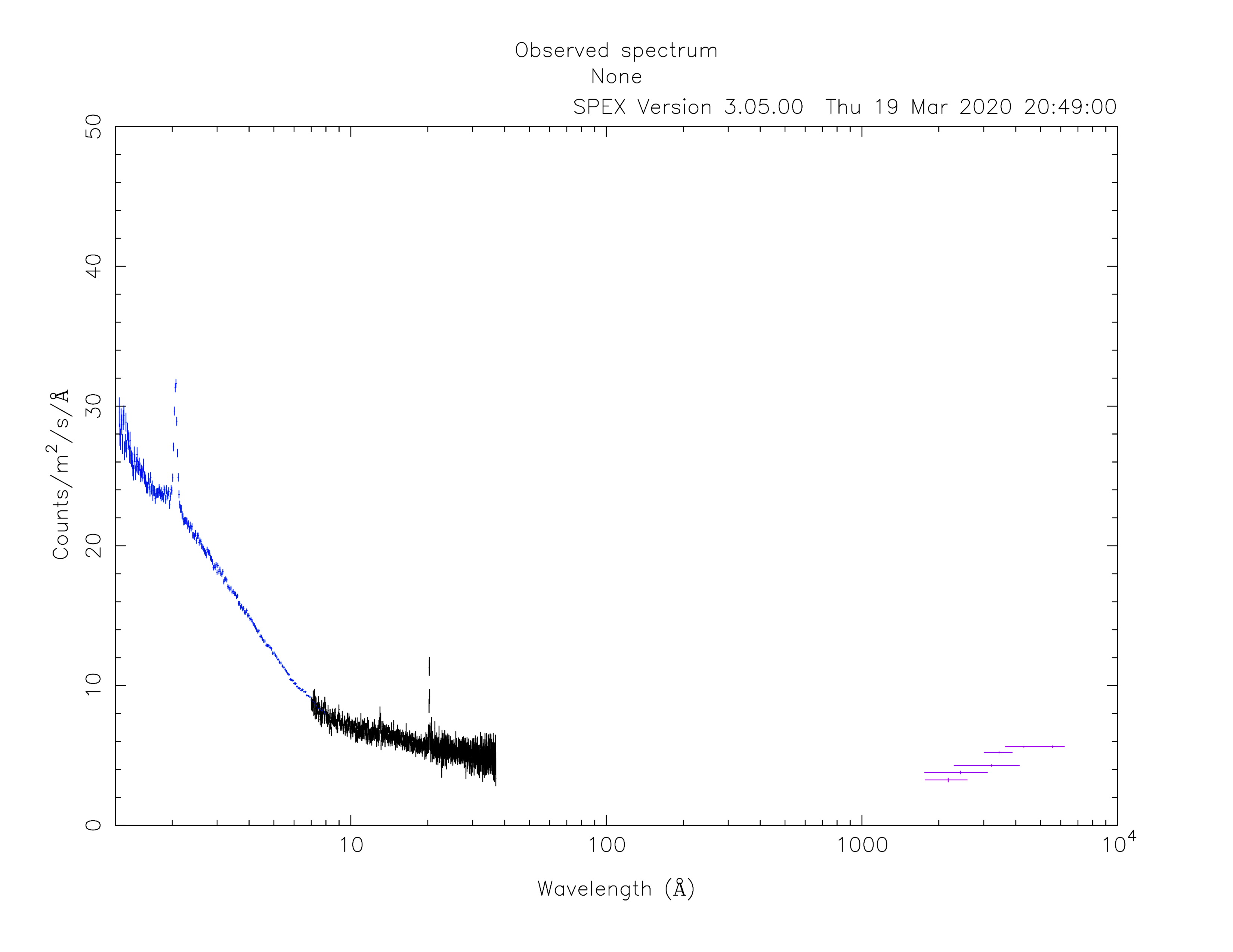
2.6.5. Plot data
plot.com is the command file tailored for this thread to plot data:
user@linux:~> cat plot.com
# plotting
plot dev xw
plot type data
plot ux a
plot uy fa
plot x log
plot rx 1.2E0 1.E4
plot y lin
plot ry 0 50
plot set 1
plot mo lw 3
plot set 2
plot da col 11
plot mo col 3
plot mo lw 3
plot set 3:8
plot da col 6
plot set all
plot back disp f
plot
Load the above command file into SPEX:
SPEX> log exe plot
2.6.6. Define model components and component relations (step-by-step)
Here we are receiving photons from three line-of-sights in a nearby (z = 0.07) Seyfert 1 galaxy.

2.6.6.1. Set the distance of the source
SPEX> dist 0.07 z
Distances assuming H0 =  70.0 km/s/Mpc, Omega_m = 0.300 Omega_Lambda = 0.700 Omega_r = 0.000
Sector       m      A.U.        ly        pc       kpc       Mpc  redshift        cz   age(yr)
----------------------------------------------------------------------------------------------
1 9.740E+24 6.511E+13 1.030E+09 3.157E+08 3.157E+05  315.6554    0.0700   20985.5 9.302E+08
----------------------------------------------------------------------------------------------
2.6.6.2. Set the redshift component
SPEX> com reds
You have defined    1 component.
SPEX> par 1 1 z val 0.07
2.6.6.3. Set the galactic absorption
SPEX> com hot
You have defined    2 components.
SPEX> par 1 2 nh val 2.0e-4
SPEX> par 1 2 t val 8E-6
SPEX> par 1 2 t s f
SPEX> par 1 2 nh s f
2.6.6.4. Set the components and component relations for line-of-sight #1
(A) Set the intrinsic spectral-energy-distribution (SED) of the AGN above the Lyman limit along line-of-sight #1.
For a typical Seyfert 1 galaxy, the SED has three components (Mehdipour et al. 2015):
A Comptonized disk component (Comt: comptonisation model) for optical to soft X-rays data
A power-law component (Pow: power law model) for X-ray data
A neutral reflection component (Refl: reflection model) for hard X-rays data. Usually, the reflection component has an exponential cut-off energy (300 keV here).
SPEX> com comt
You have defined    3 components.
SPEX> par 1 3 norm val 0.
SPEX> par 1 3 norm s f
SPEX> par 1 3 t0 val 5e-4
SPEX> par 1 3 t0 s f
SPEX> par 1 3 t1 val 0.15
SPEX> par 1 3 t1 s f
SPEX> par 1 3 tau val 20
SPEX> par 1 3 tau s f
SPEX> com pow
You have defined    4 components.
SPEX> par 1 4 norm val 1.E+09
SPEX> par 1 4 norm s t
SPEX> par 1 4 gamm val 1.7
SPEX> par 1 4 gamm s t
SPEX> com refl
You have defined    5 components.
SPEX> par 1 5 norm couple 1 4 norm
SPEX> par 1 5 gamm couple 1 4 gamm
SPEX> par 1 5 ecut val 300
SPEX> par 1 5 ecut s f
SPEX> par 1 5 pow:fgr v 0
SPEX> par 1 5 scal val 1.
SPEX> par 1 5 scal s f
(B) Apply exponential cut-off to the power-law component of the SED both below the Lyman limit and above the high-energy cut-off.
Note
The ecut parameter in the refl component applies to
itself only.
SPEX> com etau
You have defined    6 components.
SPEX> par 1 6 a val -1
SPEX> par 1 6 a s f
SPEX> par 1 6 tau val 1.3605E-2
SPEX> par 1 6 tau s f
SPEX> com etau
You have defined    7 components.
SPEX> par 1 7 a val 1
SPEX> par 1 7 a s f
SPEX> par 1 7 tau val 3.3333E-3
SPEX> par 1 7 tau s f
(C) Set the PION (obscuring wind) components.
Here we introduce two PION components for the obscuring wind (Kaastra et al. 2014). The parameters of the PION components are restricted to improve the efficiency of a realistic fitting process.
Note
The second pion component is a spare one with fcov=0
and omeg=0. This is practical when analyzing real data without any
prior knowledge of the number of PION components required.
SPEX> com pion
You have defined    8 components.
** Pion model: take care about proper COM REL use: check manual!
SPEX> com pion
You have defined    9 components.
** Pion model: take care about proper COM REL use: check manual!
SPEX> par 1 8:9 nh range 1.E-7:1.E1
SPEX> par 1 8:9 xil range -5:5
SPEX> par 1 8 nh val 5.E-02
SPEX> par 1 8 xil val 0.0
SPEX> par 1 8 zv val -3000
SPEX> par 1 8 zv s t
SPEX> par 1 8 v val 1100
SPEX> par 1 8 v s t
SPEX> par 1 9 nh val 1.E-7
SPEX> par 1 9 nh s f
SPEX> par 1 9 xil val 0
SPEX> par 1 9 xil s f
SPEX> par 1 9 fcov val 0
SPEX> par 1 9 omega val 0
(D) Set the PION (warm absorber) components.
Here we introduce three PION components for the X-ray warm absorber.
omeg=1.E-7 refers to a negligible solid angle ( ) subtended by
the PION component with respect to the nucleus (omeg =
) subtended by
the PION component with respect to the nucleus (omeg =  ).
).
Note
To see the density effect of the absorption features, it is
necessary to set a non-zero omeg value.
SPEX> com pion
You have defined    10 components.
** Pion model: take care about proper COM REL use: check manual!
SPEX> com pion
You have defined    11 components.
** Pion model: take care about proper COM REL use: check manual!
SPEX> com pion
You have defined    12 components.
** Pion model: take care about proper COM REL use: check manual!
SPEX> par 1 10:12 nh range 1.E-7:1.E1
SPEX> par 1 10:12 xil range -5:5
SPEX> par 1 10:12 omeg range 0:1
SPEX> par 1 10 nh val 5.E-03
SPEX> par 1 10 xil val 2.7
SPEX> par 1 10 zv val -500
SPEX> par 1 10 zv s t
SPEX> par 1 10 v val 100
SPEX> par 1 10 v s t
SPEX> par 1 10 omeg val 1.E-7
SPEX> par 1 11 nh val 2.E-03
SPEX> par 1 11 xil val 1.6
SPEX> par 1 11 zv val -100
SPEX> par 1 11 zv s t
SPEX> par 1 11 v val 50
SPEX> par 1 11 v s t
SPEX> par 1 11 omeg val 1.E-7
SPEX> par 1 12 nh val 1.E-7
SPEX> par 1 12 xil val 0
SPEX> par 1 12 fcov val 0
SPEX> par 1 12 omega val 0
(E) Set the component relation for line-of-sight #1.
Note
Photons from both the Comptonized disk and power-law components are screened by the obscuring wind and warm absorber components at the redshift of the target, as well as the galactic absorption before reaching the detector. Photons from the neutral reflection component is assumed not to be screened by the obscuring wind and warm absorber for simplicity. It is still redshifted and requires the galactic absorption.
SPEX> com rel 3 8,9,10,11,12,1,2
SPEX> com rel 4 6,7,8,9,10,11,12,1,2
SPEX> com rel 5 1,2
(F) Set the component relation for the PION components. Assuming that the
obscuring wind and warm absorber components closer to the central engine
are defined first (with a smaller component index), photons transmitted
from the inner PION components (with a nonzero omeg value) are screened
by all the outer PION components at the redshift of the target, as well as
the galactic absorption before reaching the detector.
SPEX> com rel 8 9,10,11,12,1,2
SPEX> com rel 9 10,11,12,1,2
SPEX> com rel 10 11,12,1,2
SPEX> com rel 11 12,1,2
SPEX> com rel 12 1,2
2.6.6.5. Set the components and component relations for line-of-sights #2 and #3
(A) Set the AGN SED above the Lyman limit along line-of-sights #2a and #3a.
Note
Here we assume that the photoionizing SED for the X-ray broad emission PION component(s) is set to be the same as that for the obscuring wind and warm absorber. This simplification assumes that the X-ray broad-line region respond to the photoionizing SED instantaneously. Because the X-ray broad-line region is typically a few lightdays away from the central engine and it has a relatively high density. On the other hand, the photoionizing SED for the X-ray narrow emission PION component(s) is set to a long-term averaged SED. This simplification assumes that the X-ray narrow-line region is in a steady state, i.e. it varies slightly around a mean value corresponding to the mean flux level over time. Because the X-ray narrow-line region is typically a few parsecs away from the central engine and it has a relatively low density. Readers are referred to Silva et al. 2016 for a detailed spectral timing study.
SPEX> com comt
You have defined    13 components.
SPEX> par 1 13 norm:type couple 1 3 norm:type
SPEX> com pow
You have defined    14 components.
SPEX> par 1 14 norm:lum couple 1 4 norm:lum
SPEX> com comt
You have defined    15 components.
SPEX> par 1 15 norm val 1.E12
SPEX> par 1 15 norm s f
SPEX> par 1 15 t0 val 3.E-4
SPEX> par 1 15 t0 s f
SPEX> par 1 15 t1 val 0.125
SPEX> par 1 15 t1 s f
SPEX> par 1 15 tau val 20
SPEX> par 1 15 tau s f
SPEX> com pow
You have defined    16 components.
SPEX> par 1 16 norm val 6.E9
SPEX> par 1 16 norm s f
SPEX> par 1 16 gamm val 1.6
SPEX> par 1 16 gamm s f
(B) Apply exponential cut-off to the above AGN SEDs at all energies because these photons do not reach us (dashed gray lines in Figure 1).
SPEX> com etau
You have defined    17 components.
SPEX> par 1 17 tau val 1.E3
SPEX> par 1 17 tau s f
SPEX> par 1 17 a val 0
SPEX> par 1 17 a s f
(C) Set the PION (emission) components.
Here we introduce three PION components. The parameters of the PION components
are restricted to improve the efficiency of a realistic fitting process.
fcov=0 for the emission PION components.
Note
The first pion component refers to the X-ray broad-line
region. The second pion component refers to the X-ray narrow-line
region. The third pion component is a spare one with fcov=0 and
omeg=0. This is practical when analyzing real data without any prior
knowledge of the number of PION components required.
SPEX> com pion
You have defined    18 components.
** Pion model: take care about proper COM REL use: check manual!
SPEX> com pion
You have defined    19 components.
** Pion model: take care about proper COM REL use: check manual!
SPEX> com pion
You have defined    20 components.
** Pion model: take care about proper COM REL use: check manual!
SPEX> par 1 16:18 nh range 1.E-7:1.E1
SPEX> par 1 16:18 xil range -5:5
SPEX> par 1 16:18 omeg range 0:1
SPEX> par 1 16 nh val 8.E-02
SPEX> par 1 16 xil val 0.8
SPEX> par 1 16 zv val 0
SPEX> par 1 16 zv s f
SPEX> par 1 16 v val 100
SPEX> par 1 16 v s f
SPEX> par 1 16 omeg val 3.E-2
SPEX> par 1 16 omeg s t
SPEX> par 1 17 nh val 5.E-02
SPEX> par 1 17 xil val 2.3
SPEX> par 1 17 zv val 0
SPEX> par 1 17 zv s f
SPEX> par 1 17 v val 240
SPEX> par 1 17 v s t
SPEX> par 1 17 omeg val 5.E-2
SPEX> par 1 17 omeg s t
SPEX> par 1 18 nh val 1.E-7
SPEX> par 1 18 nh s f
SPEX> par 1 18 xil val 0
SPEX> par 1 18 xil s f
SPEX> par 1 18 fcov val 0
SPEX> par 1 18 omeg val 0
(D) Set the broadening due to macroscopic motion for the PION (emission) components.
Note
The v parameter in PION components refer to the microscopic
(i.e. turbulent) motion. The macroscopic motion refers to the rotation
around the black hole. For the X-ray broad emission lines, the macroscopic
motion dominates the broadening. For the X-ray narrow emission lines, the
microscopic and macroscopic motion are often degenerate (Mao et al. 2018). The
second and third vgau components are spare.
SPEX> com vgau
You have defined    21 components.
par 1 21 sig val 7.E3
par 1 21 sig s t
SPEX> com vgau
You have defined    22 components.
SPEX> com vgau
You have defined    23 components.
(E) Set the component relation for line-of-sights #2a and #3a.
Note
Photons from both the Comptonized disk and power-law (with exponential low- and high-energy cut-offs) components are the photoionizing source of the PION emission components at the redshift of the target. While (reflected/reprocessed) photons from the PION emission components reach us.
SPEX> com rel 13 18,1,17
SPEX> com rel 14 6,7,18,1,17
SPEX> com rel 15 19,20,1,17
SPEX> com rel 16 6,7,19,20,1,17
(F) Set the component relation for the PION (emission) components.
Note
Here we assume that the obscuring wind is outside the X-ray broad-line region and it screens photons emitted from the X-ray broad-line region before it reaches us. On the other hand, since the obscuring wind is closer to the central engine than the X-ray narrow-line region, photons emitted from the X-ray narrow-line region are not screened by the obscuring wind.
SPEX> com rel 18 21,8,9,1,2,26
SPEX> com rel 19 22,1,2,26
SPEX> com rel 20 23,1,2,26
(G) Set the component relation for the AGN SED below the Lyman limit (optical/UV) along line-of-sight #1.
SPEX> com rel 24 30,1,31,27
SPEX> com rel 25 6,7,30,1,31,27
SPEX> com rel 28 1
SPEX> com rel 29 1
2.6.7. Check settings and calculate
We check the setting of the component relation:
SPEX> model show
--------------------------------------------------------------------------------
 Number of sectors         :     1
 Sector:    1 Number of model components:    31
    Nr.    1: reds
    Nr.    2: hot
    Nr.    3: comt[8,9,10,11,12,1,2,26 ]
    Nr.    4: pow [6,7,8,9,10,11,12,1,2,26 ]
    Nr.    5: refl[1,2,26 ]
    Nr.    6: etau
    Nr.    7: etau
    Nr.    8: pion[9,10,11,12,1,2,26 ]
    Nr.    9: pion[10,11,12,1,2,26 ]
    Nr.   10: pion[11,12,1,2,26 ]
    Nr.   11: pion[12,1,2,26 ]
    Nr.   12: pion[1,2,26 ]
    Nr.   13: comt[18,1,17 ]
    Nr.   14: pow [6,7,18,1,17 ]
    Nr.   15: comt[19,20,1,17 ]
    Nr.   16: pow [6,7,19,20,1,17 ]
    Nr.   17: etau
    Nr.   18: pion[21,8,9,1,2,26 ]
    Nr.   19: pion[22,1,2,26 ]
    Nr.   20: pion[23,1,2,26 ]
    Nr.   21: vgau
    Nr.   22: vgau
    Nr.   23: vgau
    Nr.   24: comt[30,1,31,27 ]
    Nr.   25: pow [6,7,30,1,31,27 ]
    Nr.   26: etau
    Nr.   27: etau
    Nr.   28: file[1 ]
    Nr.   29: file[1 ]
    Nr.   30: ebv
    Nr.   31: ebv
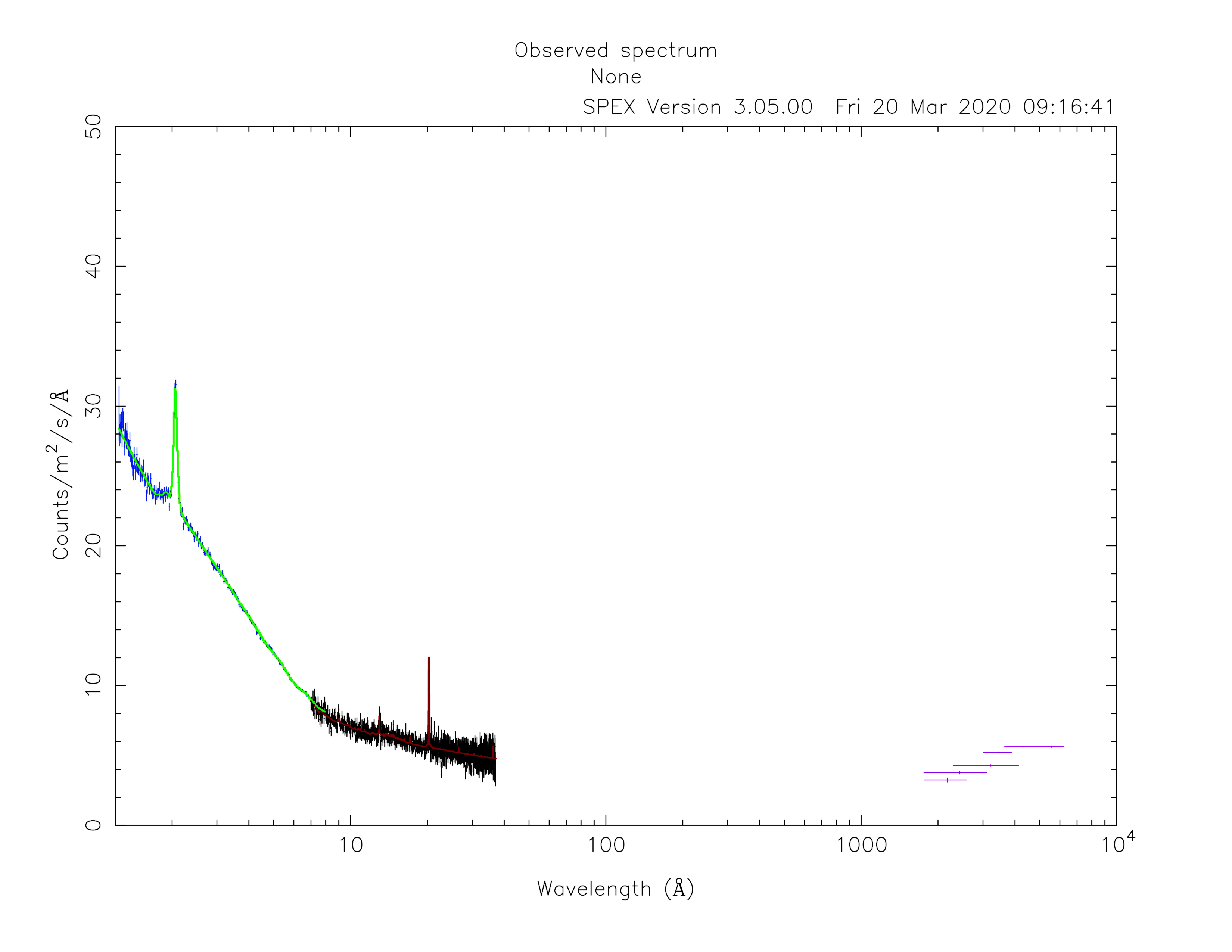
We check the setting of the free parameters and calculate the 1–1000 Ryd ionizing luminosity:
SPEX> elim 1.E0:1.E3 ryd
SPEX> calc
SPEX> plot
SPEX> par show free
--------------------------------------------------------------------------------------------------
sect comp mod  acro parameter with unit     value      status    minimum   maximum lsec lcom lpar


   1    3 comt norm Norm (1E44 ph/s/keV) 3.0000001E+12 thawn     0.0      1.00E+20
   1    3 comt t0   Wien temp (keV)      5.0000002E-04 thawn    1.00E-05  1.00E+10
   1    3 comt t1   Plasma temp (keV)    0.1500000     thawn    1.00E-05  1.00E+10
   1    3 comt tau  Optical depth         20.00000     thawn    1.00E-03  1.00E+03

   1    4 pow  norm Norm (1E44 ph/s/keV) 1.0000000E+09 thawn     0.0      1.00E+20
   1    4 pow  gamm Photon index          1.700000     thawn    -10.       10.


   1    8 pion nh   X-Column (1E28/m**2) 5.0000001E-02 thawn    1.00E-07   10.
   1    8 pion xil  Log xi (1E-9 Wm)      0.000000     thawn    -5.0       5.0
   1    8 pion v    RMS Velocity (km/s)   1100.000     thawn     0.0      3.00E+05
   1    8 pion zv   Average vel. (km/s)  -3000.000     thawn   -1.00E+05  1.00E+05


   1   10 pion nh   X-Column (1E28/m**2) 4.9999999E-03 thawn    1.00E-07   10.
   1   10 pion xil  Log xi (1E-9 Wm)      2.700000     thawn    -5.0       5.0
   1   10 pion v    RMS Velocity (km/s)   100.0000     thawn     0.0      3.00E+05
   1   10 pion zv   Average vel. (km/s)  -500.0000     thawn   -1.00E+05  1.00E+05

   1   11 pion nh   X-Column (1E28/m**2) 2.0000001E-03 thawn    1.00E-07   10.
   1   11 pion xil  Log xi (1E-9 Wm)      1.600000     thawn    -5.0       5.0
   1   11 pion v    RMS Velocity (km/s)   50.00000     thawn     0.0      3.00E+05
   1   11 pion zv   Average vel. (km/s)  -100.0000     thawn   -1.00E+05  1.00E+05


   1   18 pion nh   X-Column (1E28/m**2) 7.9999998E-02 thawn    1.00E-07   10.
   1   18 pion xil  Log xi (1E-9 Wm)     0.8000000     thawn    -5.0       5.0
   1   18 pion omeg Scaling factor emis. 2.9999999E-02 thawn     0.0       1.0

   1   19 pion nh   X-Column (1E28/m**2) 5.0000001E-02 thawn    1.00E-07   10.
   1   19 pion xil  Log xi (1E-9 Wm)      2.300000     thawn    -5.0       5.0
   1   19 pion v    RMS Velocity (km/s)   240.0000     thawn     0.0      3.00E+05
   1   19 pion omeg Scaling factor emis. 9.9999998E-03 thawn     0.0       1.0


   1   21 vgau sig  Sigma (km/s)          7000.000     thawn     0.0      3.00E+05


   1   28 file norm Flux scale factor    0.3000000     thawn     0.0      1.00E+20

   1   29 file norm Flux scale factor    0.4000000     thawn     0.0      1.00E+20

   1   30 ebv  ebv  E(B-V)  (mag)        0.1000000     thawn     0.0      1.00E+20

   1   31 ebv  ebv  E(B-V)  (mag)        0.1200000     thawn     0.0      1.00E+20


Instrument     1 region    1 has norm    1.00000E+00 and is frozen
Instrument     2 region    1 has norm    1.00000E+00 and is frozen
Instrument     3 region    1 has norm    1.00000E+00 and is frozen
Instrument     4 region    1 has norm    1.00000E+00 and is frozen
Instrument     5 region    1 has norm    1.00000E+00 and is frozen
Instrument     6 region    1 has norm    1.00000E+00 and is frozen
Instrument     7 region    1 has norm    1.00000E+00 and is frozen
Instrument     8 region    1 has norm    1.00000E+00 and is frozen

--------------------------------------------------------------------------------
 Fluxes and restframe luminosities between  1.36057E-02 and    13.606     keV

 sect comp mod   photon flux   energy flux nr of photons    luminosity
              (phot/m**2/s)      (W/m**2)   (photons/s)           (W)
    1    3 comt  7.891731E-04  1.775058E-19  1.447225E+54  7.988903E+36
    1    4 pow    38.8452      3.366349E-14  2.869709E+54  1.021578E+38
    1    5 refl   5.98573      7.190706E-15  6.284845E+51  7.467510E+36
    1    8 pion   0.00000       0.00000       0.00000       0.00000
    1    9 pion   0.00000       0.00000       0.00000       0.00000
    1   10 pion  1.755872E-08  5.460370E-24  2.240611E+44  1.101832E+28
    1   11 pion  7.849879E-10  9.871699E-26  3.169252E+45  7.940836E+27
    1   12 pion   0.00000       0.00000       0.00000       0.00000
    1   13 comt   1213.94      6.701157E-15  1.447225E+54  7.988903E+36
    1   14 pow    1657.30      8.033095E-14  2.869709E+54  1.021578E+38
    1   15 comt   0.00000       0.00000      1.106767E+53  5.268881E+35
    1   16 pow    0.00000       0.00000      1.296679E+55  6.397146E+38
    1   18 pion  2.157629E-03  5.832195E-19  1.541392E+54  9.503085E+36
    1   19 pion   3.30138      4.647512E-16  5.174083E+52  1.025305E+36
    1   20 pion   0.00000       0.00000       0.00000       0.00000
    1   24 comt  0.501314      1.089752E-18  1.447225E+54  7.988903E+36
    1   25 pow   0.193548      4.207327E-19  2.869709E+54  1.021578E+38
    1   28 file   0.00000       0.00000       0.00000       0.00000
    1   29 file   0.00000       0.00000       0.00000       0.00000

 Fit method        : Classical Levenberg-Marquardt
 Fit statistic     : C-statistic
 C-statistic       :      1215.69
 Expected C-stat   :      1212.71 +/-        49.26
 Chi-squared value :      1221.23
 Degrees of freedom:         0
 W-statistic       :         0.00
 Contributions of instruments and regions:
   Ins   Reg    Bins      C-stat  Exp C-stat  Rms C-stat      chi**2      W-stat
     1     1     996     1007.73      996.70       44.66     1012.35        0.00
     2     1     210      197.87      210.01       20.49      198.61        0.00
     3     1       1        3.06        1.00        1.41        3.22        0.00
     4     1       1        0.01        1.00        1.41        0.01        0.00
     5     1       1        0.31        1.00        1.41        0.32        0.00
     6     1       1        0.20        1.00        1.41        0.20        0.00
     7     1       1        4.62        1.00        1.41        4.67        0.00
     8     1       1        1.89        1.00        1.41        1.87        0.00

2.6.8. Final remarks
This is the end of this analysis thread. If you want, you can quit SPEX now:
SPEX> quit
Thank you for using SPEX!
Below, we provide a useful command file.
2.6.8.1. Define model components and component relations (running scripts)
calc.com is the command file tailored for this thread.
Load the above command file into SPEX:
user@linux:~> spex
Welcome user to SPEX version 3.05.00

SPEX> log exe calc